Distributed Graph Matching and Graph Indexing Approaches

Applications to Pattern Recognition

Zeina Abu-Aisheh, Romain Raveaux and Jean-Yves Ramel

Laboratoire d’Informatique (LI), Universit

e Franc¸ois Rabelais, 37200, Tours, France

Keywords:

Graph Matching, Graph Edit Distance, Pattern Recognition, Classiﬁcation, Distributed Systems, Scalability.

Abstract:

Attributed graphs are powerful data structures for the representation of complex objects. In a graph-based

representation, vertices and their attributes describe objects (or part of objects) while edges represent interre-

lationships between the objects. Due to the inherent genericity of graph-based representations, and thanks to

the improvement of computer capacities, structural representations have become more and more popular in the

ﬁeld of Pattern Recognition (PR). In this thesis, we tackle two important graph-based problems for PR: Graph

Matching and Graph Indexing. The comparison between two objects is a crucial operation in PR. Represent-

ing objects by graphs turns the problem of object comparison into graph matching where correspondences

between nodes and edges of two graphs have to be found. Moreover, graph-based indices are important so that

a graph query can be retrieved from a large database via such indices, such a problem is referred to as graph in-

dexing. The complexity of both graph matching and graph indexing is generally stated to be NP-COMPLETE

or NP-hard. Coming up with a graph matching algorithm that can scale up to match graphs involved in PR

tasks is a great challenge. Among the graph matching methods dedicated to PR problems, the Graph Edit

Distance (GED) is of great interest. Over the last decade, GED has been applied to a wide range of speciﬁc

applications from molecule recognition to image classiﬁcation. In this report, we present the ﬁrst part of the

thesis. We tackle GED, shed light on the importance of having exact solutions rather than approximate ones

and come up with a distributed GED where the search tree is decomposed into smaller trees which are solved

independently and in a complete distributed manner. In the second part of the thesis, we aim at proposing new

distributed graph-indexing approaches that aim at retrieving a graph from a large graph-based index as fast as

possible. Graph indexing will be reported as a perspective of this work.

1 INTRODUCTION

Graphs are an efﬁcient data structure for structural ob-

jects representation. Over the last decades, much at-

tention has been shed on using graphs as a structural

representation of objects in Pattern Recognition (PR).

In PR, the attributes of both nodes and edges play

an important role for representing graphs. Combin-

ing both symbolic and numeric attributes on nodes

and edges makes the extracted nodes and edges more

meaningful and highly representative. Unlike the

other graphs used in other ﬁelds (e.g., shortest path)

where the combination of symbolic and numeric at-

tributes is not necessarily needed. Representing ob-

jects by graphs easily transforms the problem of ob-

ject detection or objects comparison into a graph

matching one.

Graph matching is the process of ﬁnding a corre-

spondence between the nodes and the edges of two

graphs g

and g

that satisﬁes some (more or less

stringent) constraints ensuring that similar substruc-

tures of the source graph are mapped to similar sub-

structures of the target graph. Recently, graph match-

ing has been considered as a fundamental problem in

PR. Such a problem is known to be NP-complete, ex-

cept for graph isomorphism, for which it has not yet

been demonstrated whether it belongs to NP or not

(Conte et al., 2004).

Exact graph matching addresses the problem of

detecting identical (sub)structures of two graphs g

and g

and their corresponding labels. This category

assumes the existence of only noise-free objects while

in reality objects are usually affected by noise and

distortion. Consequently, researchers often shed light

on the other category, i.e., inexact or so-called error-

tolerant graph matching, where some degree of er-

ror tolerance can be easily integrated into the graph

matching process.

In the context of attributed graphs, the problem

of error tolerant graph matching presents a higher

Abu-Aisheh Z., Raveaux R. and Ramel J..

Distributed Graph Matching and Graph Indexing Approaches - Applications to Pattern Recognition.

 2015 SCITEPRESS (Science and Technology Publications, Lda.)

complexity than exact graph matching as it takes dis-

tortion and noise into account during the matching

process. Indeed, the exact algorithms dedicated to

solving error-tolerant graph matching are computa-

tionally complex (Vento, 2014); and (M. Neuhaus

and Bunke., 2006)). Consequently, lots of works

have been employed to approximately solve the error-

tolerant graph matching problem. Such methods are

often called heuristics or approximate methods. Ap-

proximate methods for the error-tolerant graph match-

ing problem have been investigated based on genetic

algrithm (A.D.J. Cross and Hancock, 1997), proba-

bilistic relaxation (W. Christmas and Petrou., 1995),

EM algorithm (Andrew D. J. Cross, 1998); (Finch,

1998) and neural networks (Kuner and Ueberreiter,

1988). The aforementioned techniques are expected

to present a polynomial run-time. However, they can-

not ensure the quality of their solutions and are likely

to output suboptimal solutions.

Graph Edit Distance, referred to as GED, is an

error-tolerant technique that has been widely studied

and largely applied to PR (Tsai and Fu, 1979). Its

ﬂexibility comes from its generality as it is applicable

on unconstrained attributed graphs. GED is a general-

ization of the graph isomorphism problem where the

goal is to minimize the cost of graph transformation.

In GED, graph g

is transformed into graph g

means of series of transformations. The allowed edit

operations are: deletion, insertion and substitution of

nodes and their corresponding edges. GED is compu-

tationally complex or expensive, it is said to be an NP-

COMPLETE problem where the complexity is expo-

nential in the number of nodes of the involved graphs.

Such a fact limits GED algorithms to work on rela-

tively small graphs. To overcome this problem three

main directions have been adopted in the literature.

First, optimal methods based on admissible heuristics

to prune the search space (e.g., (Riesen et al., 2007)).

Second, sub-optimal methods simplifying the prob-

lem (e.g., (M. Neuhaus and Bunke., 2006)). Third,

sub-optimal methods by means of approximate op-

timization algorithm (e.g., (Riesen, 2009); and (An-

dreas Fischer, 2013)). However, sub-optimal meth-

ods does not guarantee to ﬁnd the best matching and

the error rate gets higher as the involved graphs get

larger. Accordingly, in this thesis a focus is given to

optimal methods. To prevent the combinatorial ex-

plosion, many works have been focused on efﬁciently

pruning the search space. The computation of ad-

missible lower bounds have been deeply studied to

reduce memory and CPU complexity (Bunke, 1983);

and (Zeng et al., 2009).

Most of the current techniques are optimized for

centralized graph processing. A distributed approach

providing horizontal scalability is required in order to

handle the analysis workload. Thus, besides provid-

ing lower and upper bounds for the problem, we have

adopted the idea of decomposing GED into smaller

problems, or sub-problems, via a divide and conquer

strategy. The sub-problems are then solved in a dis-

tributed manner.

The rest of this report is organized as follows. In

Section 2, a focus on the related works is given. In

Section 3 the notations and the deﬁnitions used in the

paper are presented and our approach is positioned

up in the literature. Section 4 reports our proposed

sequential algorithm used to solve GED. In Section

5, the chosen parallel computing model and the pro-

posed distributed GED are presented, respectively. In

Section 6 the databases and the experimental protocol

used to point out the performance of the proposed ap-

proaches are represented. Section 7 demonstrates the

results achieved so far. Finally, conclusions are drawn

and future perspectives are discussed in Section 8.

2 RELATED WORKS

The distributed and parallel graph matching methods,

presented in the literature, can be divided into two cat-

egories: Data-Parallelism and Search-Parallelism. In

Data-Parallelism, the graphs g

and g

can be parti-

tioned into sub-graphs. These small sub-graphs can

be matched independently in a sequential or in a par-

allel manner. The results of all the sub-problems

are reassembled producing a global answer of the

main graph matching problem ((Qiu and Hancock,

2006); (Patwary et al., 2010); and (Kollias, 2012)). In

Search-Parallelism, matching g

and g

is considered

as a single problem. However, the search space of g

and g

is partitioned and then processed in a com-

pletely parallel manner ((Allen and Yasuda, 1997);

(Wan, 1998); and (Plantenga, 2013)).

We focus on two distributed works, belonging to

the Search-Parallelism category and are dedicated to

solving graph matching problems:

2.1 Maspar-SIMD

A parallel inexact graph matching algorithm is pro-

posed in [22]. This algorithm, referred to as MasPar-

SIMD, is depth-ﬁrst branch-and-bound for determin-

ing a minimum-distance correspondence between two

unlabeled graphs. The heuristic, called forward

checking, used to prune the search space, examines

the possible sources of edges mismatches and thus

forward checking keeps track of constraints (edges)

that are not satisﬁed. The degree of mismatch of a

ICPRAM2015-DoctoralConsortium

permutation π is deﬁned of as the number of edges

in g

that are not mapped by π to edges in g

plus

the number of edges in g

not mapped to edges in

. At each iteration, the edge errors are accumu-

lated. Results show that MasPar-SIMD consistently

outperforms the sequential version when the involved

graphs have more than 16 vertices. This algorithm is

inexact for two reasons. First, the mismatch of edges

are taken into account whereas mismatch of nodes are

ignored. Second, the heuristic is not a lower bound

and cannot ensure the optimal solution to be found.

Also, the graphs involved in the algorithm are unla-

beled and thus numeric and attributed graphs are not

included. As for the exploration of the search space,

the best permutation and the best degree of match are

only updated at the end of each iteration, such a fact

does not allow pruning the search space as fast as pos-

sible.

2.2 SGIA-MR

Recently, a Hadoop MapReduce implementation for

subgraph type isomorphism, called SGIA-MR, has

been implemented in (Plantenga, 2013). This algo-

rithm makes use of an implicit multi-partite graph

which ﬁnds sub-graphs in a single large graph (i.e.,

given a pattern G

, ﬁnd all the walks in the graph G

that correspond to the pattern G

In (Plantenga, 2013), the type-isomorphism match

is inexact in the sense that matched subgraphs do

not necessarily have isomorphic structures. SGIA-MR

only considers symbolic or unlabeled graphs and thus

it cannot be easily extended to work on numeric at-

tributed graphs. Moreover, this algorithm is a noise-

free one as neither nodes nor edges distortion is in-

cluded in the matching process.

2.3 Conclusion on Parallel and

Distributed Graph Matching

Methods

To our best of knowledge, none of the parallel and

distributed graph matching methods has included nu-

meric attributed graphs, besides that all of them fall

within the suboptimal graph matching category and so

they cannot ensure the optimal solution to be found.

Moreover, neither bounds on the optimal solution nor

quality measure or conﬁdence on the solution are pro-

vided. In the literature, there is also no effort devoted

to solving GED problems in a distributed manner. In-

deed, MasPar-SIMD and SGIA-MR cannot be easily

extended to solve GED. We believe that there is a need

for a distributed and optimal GED method that can be

used to match symbolic and numeric attributed graphs

in a way that outperforms the sequential GED algo-

rithms.

3 GRAPH EDIT DISTANCE

Graph edit distance (GED) is a graph matching ap-

proach whose concept was ﬁrst reported in (Sanfeliu

and Fu, 1983). The basic idea of GED is to ﬁnd the

best set of transformations that can transform graph g

into graph g

by means of edit operations on graph g

The allowed operations are inserting, deleting and/or

substituting vertices and their corresponding edges.

Deﬁnition 1. Graph Edit Distance

Let g

= (V

, E

, µ

, ζ

) and g

= (V

, E

, µ

, ζ

) be

two graphs, the graph edit distance between g

and g

is deﬁned as:

GED(g

, g

) = min

,···,e

∈γ(g

)

∑

i=1

c(e

) (1)

Where c denotes the cost function measuring the

strength c(e

) of an edit operation e

and γ(g

, g

) de-

notes the set of edit paths transforming g

into g

A standard set of edit operations is given by inser-

tions, deletions and substitutions of both vertices and

edges. We denote the substitution of two vertices u

and v by (u → v), the deletion of node u by (u → ε)

and the insertion of node v by (ε → v). For edges (e.g.,

w and z), we use the same notations used for vertices.

A complete edit path (EP) refers to an edit path

that fully transforms g

into g

(i.e., complete solu-

tion). Mathematically, EP = {e

}

i=1

. An example of

an edit path between two graphs g

and g

is shown in

Figure 1, the following operations have been applied

in order to transform g

into g

: three edge deletions,

one node deletion, one node insertion, one edge inser-

tions and three node substitutions.

Figure 1: Transforming g

into g

by means of edit opera-

tions. Note that vertices attributes are represented in differ-

ent gray scales.

Many fast heuristic methods have been proposed

in the literature such as (W. Christmas and Petrou.,

1995); (Zeng et al., 2009); (Fankhauser et al., 2012);

(Combier et al., 2013); and (Andreas Fischer, 2013).

However, these heuristic algorithms can only ﬁnd un-

bounded suboptimal values. On the other hand, only

few exact approaches have been proposed to postpone

the graph size restriction (Tsai and Fu, 1979); (Justice

DistributedGraphMatchingandGraphIndexingApproaches-ApplicationstoPatternRecognition

and Hero, 2006); and (Riesen et al., 2007). Lots of

exact branch and bound graph matching algorithms

have been proposed in the literature. However, to

the best knowledge of the authors these works have

not addressed the GED problem and cannot be eas-

ily extended to solve such a problem. For instance,

a branch and bound algorithm dedicated to solving

GED was proposed in (Tsai and Fu, 1979) but it was

restricted to graphs that are structurally isomorphic.

Afterwards, this work has been extended in (Tsai and

Fu, 1983) that has taken into account insertion and

deletion of nodes and edges. However, the proposed

algorithm was devoted to error-correcting subgraph

isomorphism.

3.1 Exact Graph Edit Distance

Computation

A widely used method for exact GED computation

is based on the A* algorithm (Riesen et al., 2007),

this algorithm, referred to as A*GED, is considered

as a foundation work for solving GED. A*GED ex-

plores the space of all possible mappings between two

graphs by means of an ordered tree. Such a search

tree is constructed dynamically at run time by itera-

tively creating successor nodes linked by edges to the

currently considered node in the search tree. In the

worst case, the space complexity can be expressed as

O(|σ|) (Cormen et al., 2009) where |σ| is the cardi-

nality of the set of all possible edit paths. Since |σ|

is exponentional in the number of vertices involved in

the graphs, the memory usage is still an issue.

Algorithm 1 depicts the A*GED computation. In

order to determine the node which will be used for

further expansion of the actual mapping in the next

iteration, a heuristic function added to the actual edit

path cost is usually used. Formally, for a node p in

the search tree, g(p) represents the cost of the edit

path accumulated so far, h(p) denotes the estimated

costs from p to a leaf node, h(p) must not underes-

timate the remaining cost in order to guarantee the

optimality of the ﬁnal solution. Also, it should be

done in a faster way than the exact computation and

return a good approximation of the true future cost.

The sum g(p) +h(p), referred to as lb(p), depicts the

total cost assigned to an open node in the search tree.

Obviously, the edit path p that minimizes g(p) +h(p)

is chosen next for further expansion. Note that the

smaller the difference between lb and the real future

cost, the fewer the expanded nodes. The choice of lb

is a crucial parameter and many lower bounds have

been proposed in the literature. To the best of the

authors’ knowledge, the best lower bound has been

presented in (Riesen, 2009). In A*GED, h(p) is com-

Algorithm 1 : Astar Graph Edit Distance algorithm

(A*GED).

Input: Non-empty attributed graphs g

, E

, µ

, v

) and g

= (V

, E

, µ

, v

) where V

= {u

, ..., u

} and V

= {u

, ..., u

}

Output: A minimum cost edit path from g

to g

e.g.,

min

={u

→ v

, u

→ ε , ε → v

}

1: Initialize OPEN to the empty set

2: For each node w ∈ V

, insert the substitution in-

sert the substitution {u

→ w} into OPEN

3: Insert the deletion {u

→ ε} into OPEN

4: while true do

5: Find p

min

= argmin{g(p) + h(p)} s.t. p ∈

OPEN

6: Remove p

min

from OPEN

7: if p

min

is a complete edit path then

8: Return p

min

as the solution (i.e., a mini-

mum cost edit distance from g

to g

)

9: else

10: Let p

min

= {u

→ v

, ..., u

→ v

}

11: if k < |V

| then

12: For each w ∈ V

\ {v

, ..., v

}, insert

min

∪ {u

k+1

→ w} into OPEN

13: p

new

= {p

min

, u

k+1

→ ε}

14: Insert p

new

into OPEN

15: else

16: Insert p

min

∪

w∈V 2\{v

,...,v

}

{ε → w}

into OPEN

17: end if

18: end if

19: end while

puted using an assignment algorithm on un-

mapped vertices and edges yet to estimate the

future costs. This is performed by an assign-

ment algorithm (Riesen, 2009) whose complexity is

O(max{n

, n

}

). The unprocessed edges of both

graphs are handled analogously. Obviously, this pro-

cedure allows multiple substitutions involving the

same vertex or edge and, therefore, it possibly rep-

resents an invalid way to edit the remaining part of g

into the remaining part of g

. However, the estimated

cost certainly constitutes a lower bound of the optimal

cost.

3.2 Conclusion on A*-GED

A*GED is a best-ﬁrst search algorithm and so the list

of candidate solutions, called OPEN, grows quickly.

Such a fact leads to high memory consumption and

thus is considered as a bottleneck of A*GED. In this

paper, we outperform A*GED by getting rid of high

memory consumption and the re-computation of ver-

tices and nodes matching costs. We propose a new al-

ICPRAM2015-DoctoralConsortium

gorithm that reduces the used memory space using a

different exploration strategy (i.e., depth-ﬁrst instead

of best-ﬁrst). This approach also reduces the com-

putation time as the unfruitful nodes are pruned by

the lower and upper bounds strategy. A preprocessing

strategy is included. First, edges and vertices costs

matrices are constructed to get rid of re-computation

when exploring nodes in the search tree. Second, the

list V

is sorted to speed up the search for the best edit

path to be explored.

4 OUR SEQUENTIAL PROPOSAL

In this section, we introduce our proposal and we

mention its advantages over A*GED.

4.1 Depth-ﬁrst Graph Edit Distance

As mentioned before, A*, with all its different lower

bounds, suffers from a high memory consumption

while searching for the best edit path. A*, which

is a best-ﬁrst search algorithm, constructs the search

tree dynamically at run time. The construction of the

search tree is achieved iteratively by creating succes-

sor nodes linked by edges to the currently considered

node in the search tree.

In order to get rid of the high memory consump-

tion and to converge faster to the optimal solution,

we propose a depth-ﬁrst GED (DF). This strategy has

O(|V

|) space complexity in the worst case for stor-

ing the pending edit paths in the set OPEN (Cormen

et al., 2009). That is, at any time t the number of

pending nodes is relatively small and thus there is no

high memory consumption as in A*.

The elements of the algorithm are described in

Sections 4.2 to 4.7. Moreover, a pseudo-code for the

method is presented in Section 4.8.

4.2 Structure of Search-tree Nodes

From now on, we will refer to the search-subtree

rooted in node p as Partial Edit Path (p). Figure 2

illustrates an example of a partial edit path.

Each p is then identiﬁed by the following ele-

ments:

• matched-vertices(p) and matched-edges(p): the

elements contained in these sets are vertices and

edges that have been matched so far in both g

and g

. These sets can contain substitution (u →

v), deletion (u → ε) and/or insertion (ε → v) of

vertices and edges, correspondingly.

b c d

g(a)=0

lb(a)=4

f(a)=4

g(d)=4

lb(d)=4

f(d)=8

g(c)=2

lb(c)=1

f(c)=3

g(b)=2

lb(b)=2

f(b)=4

g(e)=5

lb(e)=1

F(e)=6

g(f)=4

lb(f)=1

f(f)=5

Figure 2: An example of a partial edit path p whose ex-

plored nodes so far are a, c and f . f (∗) = g(∗) + h(∗).

• pending-vertices

(p) and pending-edges

(p):

these sets represent vertices and edges of both

and g

(i.e., V

, V

, E

and E

) that are

not substituted, deleted or inserted yet where

pending-vertices

(p) and pending-vertices

(p)

represent pending V

and pending V

, respectively

whereas pending-edges

(p) and pending-

edges

(p) represent pending E

and pending E

respectively.

• parent(p): the parent of p.

• siblings(p): for any node p, the exploration is

achieved by choosing the next most promising

vertex u

of pending-vertices

(p) and matching it

with all the elements of pending-vertices

(p) in

addition to the deletion of this node (i.e., u

→ ε).

All these matchings are referred to as siblings(p).

• h(p): is the estimated future cost from node p.

h(p) does not underestimate the complete solu-

tion. The calculation of h(p) is described in Sec-

tion 4.6.

• g(p): the cost of matched-vertices(p) and

matched-edges(p). Both h and g depend on the

attributes as well as the structure of the involved

sub-trees. The cost functions involved with each

PR dataset permit to calculate insertions, dele-

tions and substitutions of vertices and/or edges.

4.3 Preprocessing

Preprocessing is applied before the branch and bound

procedure starts in order to speed up the tree search

exploration. First, vertices and edges cost matri-

ces are constructed. Second, vertices-sorting is con-

ducted.

4.3.1 Cost Matrices

The vertices and edges cost matrices (C

and C

) are

constructed, respectively. This step aims at speeding

up branch and bound by getting rid of re-calculating

the assigned costs when matching vertices and edges

of g

and g

DistributedGraphMatchingandGraphIndexingApproaches-ApplicationstoPatternRecognition

Let g

= (V

, E

, µ

, ξ

) and g

= (V

, E

, µ

, ξ

)

be two graphs with V

= (u

, ..., u

) and V 2 =

, ..., v

). A vertices cost matrix C

, whose dimen-

sion is (n + 2) X (m + 2), is constructed as follows:

1,1

... ... c

1,m

1←ε

1→ε

... ... ... ... ... ...

n,1

... ... c

n,m

n←ε

n→ε

ε→1

... ... c

ε→m

∞ ∞

ε←1

... ... c

ε←m

∞ ∞

where n is the number of vertices of g

and m is

the number of vertices of g

Each element c

i, j

in the matrix C

corresponds to

the cost of assigning the i

vertex of the graph g

the j

vertex of the graph g

. The left upper corner

of the matrix contains all possible node substitutions

while the right upper corner represents the cost of all

possible vertices insertions and deletions of vertices

of g

, respectively. The left bottom corner contains

all possible vertices insertions and deletions of ver-

tices of g

, respectively whereas the bottom right cor-

ner elements cost is set to inﬁnity which concerns the

substitution of ε − ε.

Similarly, C

contains all the possible substitu-

tions, deletions and insertions of edges of g

and g

is constructed in the very same way as C

4.3.2 Vertices-Sorting Strategy

As GED aims at transforming g

into g

so it is impor-

tant to sort V

in order to start with the most promis-

ing vertices that will speed up the exploration of the

search tree while searching for the optimal solution.

The aforementioned C

is used as an input of the

vertices-sorting phase. To sort V

, Munkres’ algo-

rithm is applied (Riesen, 2009). From now on, we

will refer to the set of sorted vertices as sorted-V

4.4 Branching Strategy

A systematic evaluation of all possible solutions is

performed without explicitly evaluating all of them.

The solution space is organized as an ordered tree

which is explored in a depth-ﬁrst way. In depth-ﬁrst

search, each node is visited just before its siblings.

In other words, when traversing the search tree, one

should travel as deep as possible from node i to node

j before backtracking.

The root r of the search-tree is the node with

matched-vertices(r) = φ, matched-edges(r) = φ,

pending-vertices

1,2

(r) = V

∪V

, pending-edges

1,2

(r)

= E

∪ E

, g(r) = ∞ and lb(r) = ∞. Initially r is the

only node in the set OPEN; the set of the edit paths,

found so far. The exploration starts with the ﬁrst most

promising vertex u

in sorted-V

in order to gener-

ate the root’s siblings siblings(r). Then, siblings(r) is

added to OPEN. Consequently, a minimum edit path

min

) is chosen to be explored by selecting the min-

imum cost node (i.e., min(lb(p)) among siblings(r)

and so on. We backtrack to continue the search for a

good edit path by revoking p

min

(if p

min

equals null)

and trying out the next child in the set of siblings(r)

and so on.

4.5 Reduction Strategy

As in A*, pruning, or bounding, is achieved thanks to

h(p), g(p) and a global upper bound UB obtained at

node leaves. Formally, for a node p in the search tree,

the sum g(p) + h(p) is taken into account and com-

pared with UB. That is, if g(p) + h(p) is less than U B

then p can be explored. Otherwise, the encountered

p will be pruned from OPEN and a backtracking is

done looking for the next promising node and so on

until ﬁnding the best UB that represents the optimal

solution of DF-GED. This algorithms differs from

A* as at any time t, in the worst case, OPEN con-

tains approximately |V

|.|V

| elements and hence the

memory consumption is not exhausted.

4.6 Lower Bound

The lower bound lb(p), adapted to DF-GED, is the

one used in section A*GED, see Section 3.1.

4.7 Upper Bound

The very ﬁrst upper bound is computed by Munkres’

algorithm as it provides fast preliminary results on the

GED problem, see (Riesen, 2009) for more details.

Afterwards and while traversing the search tree, the

upper bound UBCOST is replaced by the best UB-

COST found so far (i.e., a complete path whose cost

is less than the current UBCOST). After ﬁnishing the

traversal of the search tree (i.e., when p

min

is empty

and its parent is r), the best UBCOST is outputted

as an optimal solution of DF. Encountering upper

bounds when performing a depth-ﬁrst traversal efﬁ-

ciently prunes the search space and thus helps at ﬁnd-

ing the optimal solution faster than A*.

4.8 Pseudo Code

As depicted in Algorithm 2, DF-GED starts by a pre-

processing step (line 2), then an upper bound UB-

COST is calculated by BP (line 3). The traversal of

ICPRAM2015-DoctoralConsortium

Algorithm 2: Depth-ﬁrst GED algorithm (DF-GED).

Input: Non-empty attributed graphs g

, E

, µ

, v

) and g

= (V

, E

, µ

, v

) where V

= {u

, ..., u

} and V

= {u

, ..., u

}

Output: A distance UBCOST and a minimum cost

edit path (UB) from g

to g

e.g., {u

→ v

, u

→ ε

, ε → v

}

1: OPEN ← {φ}, p

min

← φ

2: Generate C

, C

and sorted-V

3: (U B , UBCOST) ←BP(g

)

4: for w ∈ V

5: OPEN ← OPEN ∪{u

→ w} s.t. u

∈ sorted-

6: end for

7: OPEN ← OPEN ∪ {u

→ ε}

8: r ← parent(u

), parent

tmp

← r

9: while true do

10: p

min

← bestSibling(parent

tmp

)

11: while p

min

is not empty and parent

tmp

does

not equal to r do

12: parent

tmp

← backtrack(parent

tmp

)

13: p

min

← bestSibling(parent

tmp

)

14: end while

15: if p

min

is empty and parent

tmp

equals to r then

16: Return UB and UBCOST

17: end if

18: OPEN ← OPEN \ p

min

19: if g(p

min

) + h(p

min

) < UB then

20: if pending-vertices

min

) is not empty

then

21: for w ∈ pending-vertices

min

) do

22: p ← p

min

∪ {u

k+1

→ w}

23: if g(p) + h(p) <UBCOST then

24: OPEN ← OPEN ∪ {p}

25: end if

26: end for

27: p ← p

min

∪ {u

k+1

→ ε}

28: if g(p) + h(p) <UBCOST then

29: OPEN ← OPEN ∪ {p}

30: end if

31: else

32: Generate a complete solution p ←

min

∪

w∈pending−vertices

(p)

{ε → w}

33: if g(p) + h(p) <UBCOST then

34: UBCOST ← g(p)

35: UB ← p

36: end if

37: end if

38: end if

39: parent

tmp

← p

min

40: end while

the search tree starts by selecting a ﬁrst vertex

∈ sorted-V

where u

substituted with all vertex

w in graph g

as well as the deletion case (u

→ ε)

are inserted into OPEN (lines 4 to 7). A branching

step is performed in line 10 where the best sibling

min

is selected, the backtracking is done when there

is no more siblings to explore in the selected branch

and the parent node (parent

tmp

) is not the root (lines

11 to 14). p

min

is explored by substituting the next

promising node u

k+1

with pending-vertices

min

)

and also deleting u

k+1

, respectively (lines 20 to 30).

Similar to A*GED, if pending-vertices

min

) is

empty, pending-vertices

min

) will be inserted (line

32). UB and UBCOST are updated whenever a better

UBCOST is encountered (lines 34 and 35). Each

time the next parent to be explored will be replaced

by p

min

(line39). This algorithm guarantees to ﬁnd

the optimal solution of GED(g

, g

). Note that edges

operations are taken into account in the matching

process when substituting, deleting or inserting their

corresponding vertices.

4.9 Deadlocks to be Released

DF-GED ends up ﬁnding the optimal edit path be-

tween two graphs. However, its bottleneck comes

from its CPU consumption. Indeed, DF-GED is com-

putationally complex as the size of the search space

increases exponentially with the number of nodes of

the involved graph. Such facts restrict it to work on

small graphs only. On the other hand, approximate

methods often have a polynomial running time in the

size of the input graphs which is much faster, but are

not guaranteed to ﬁnd the optimal solution. We, au-

thors, believe that the more complex the graphs, the

larger the error committed by the approximate meth-

ods. The graphs are more complex when they have

more vertices and a well-connected structure. For

all these reasons we shed light on the necessity of

having a distributed DF-GED in order to work on

larger graphs that cannot be matched using DF-GED.

Scaling-out is essential and ﬂexible as one can add M

machines for enhancing the execution time.

5 OUR DISTRIBUTED

PROPOSAL

Recently, people have been increasingly ﬂooding onto

deploying their applications on servers which respond

to more complicated requirements: scalability, pro-

ductivity and performance. To respond to this de-

mand, an application server is proposed in this re-

search. We present a distributed DF-GED algorithm,

denoted by D-DF. This proposed algorithm is built

DistributedGraphMatchingandGraphIndexingApproaches-ApplicationstoPatternRecognition

on top of Hadoop-MapReduce. The search tree is de-

composed into smaller trees, or sub-trees and the ex-

ploration of the partial edit paths is done in parallel.

Deﬁnition 2. Scalability

The capability of a system or a process to handle a

growing amount of work, e.g., larger graphs, or to be

easily expanded or upgraded, when required, to ac-

commodate that amount of work. This is done by

adding more machines to the distributed system.

For the sake of programming ease, we have cho-

sen MapReduce as a model on which we build our dis-

tributed approach. MapReduce is easier to program,

even for programmers who have no much background

about parallel computing as it hides the details of par-

allelization, fault-tolerance, data distribution and load

balancing from them.

5.1 MapReduce Framework

MapReduce is a GOOGLE parallel computing frame-

work (Dean, 2004) used to process vast amounts of

data in-parallel. In the MapReduce model, the work

is divided into two phases: a Map phase and a Re-

duce phase. Both of these phases work on key-value

pairs. These pairs are deﬁned by the MapReduce pro-

grammers depending on the problems they are han-

dling (e.g., words in a text paired by their number of

occurrences).

DF-GED is a data-intensive task where lots of edit

paths are extracted searching for a best complete edit

path to transform g

into g

. MapReduce is a Single

Program Multiple data (SPMD) model, dedicated to

data-intensive tasks. As a consequence, such a par-

allel computing model suits DF-GED, thanks to its

scalability and its ability to be run on a large cluster

of machines.

Deﬁnition 3. Job

A MapReduce job contains a Map procedure and a

Reduce procedure. Each procedure has one or more

workers (i.e., Map or Reduce workers that are as-

signed to Map or Reduce tasks, respectively). Map

and Reduce tasks are run by their workers in parallel.

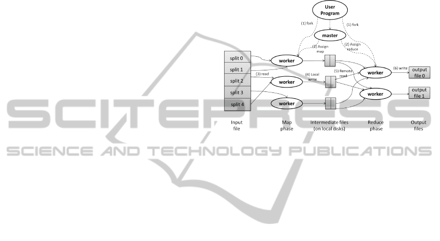
MapReduce uses ﬁle-systems as a communication

way between Map and Reduce functions. In other

words, MapReduce programs read and write theirs re-

sults to disks. Figure 3 represents a MapReduce job.

In MapReduce, the input ﬁles are split into N pieces,

or splits, by the MapReduce library in the user pro-

gram. Then the master, which has a special copy of

the program, assigns Map and Reduce tasks to Map

workers and Reduce workers, respectively. Each Map

worker is assigned one or more ﬁle splits (i.e., one or

more map tasks), depending on its idleness. When

a Map worker ﬁnishes its associated task, it saves its

buffered key-value pairs to the local disk. The local

locations of these buffers are sent back to the master

which will inform Reduce workers about them when

all the Map workers ﬁnish their assigned tasks. Re-

duce workers read these buffers from their locations,

group data by their keys and start to execute the Re-

duce function.

Figure 3: MapReduce Job (Dean, 2004).

5.2 Architecture

The time complexity of DF-GED is exponential in the

number of vertices of the involved graphs (i.e., g

and

), in order to decrease the execution time of DF-

GED, a search tree decomposition is proposed here

to fragment the graph matching problem into smaller

problems that are solved in a parallel manner. We re-

fer to this distributed approach as D-DF. D-DF has

a single job that has a Map phase without a Reduce

one. It starts with two graphs g

and g

and ends up

ﬁnding the optimum distance (d).

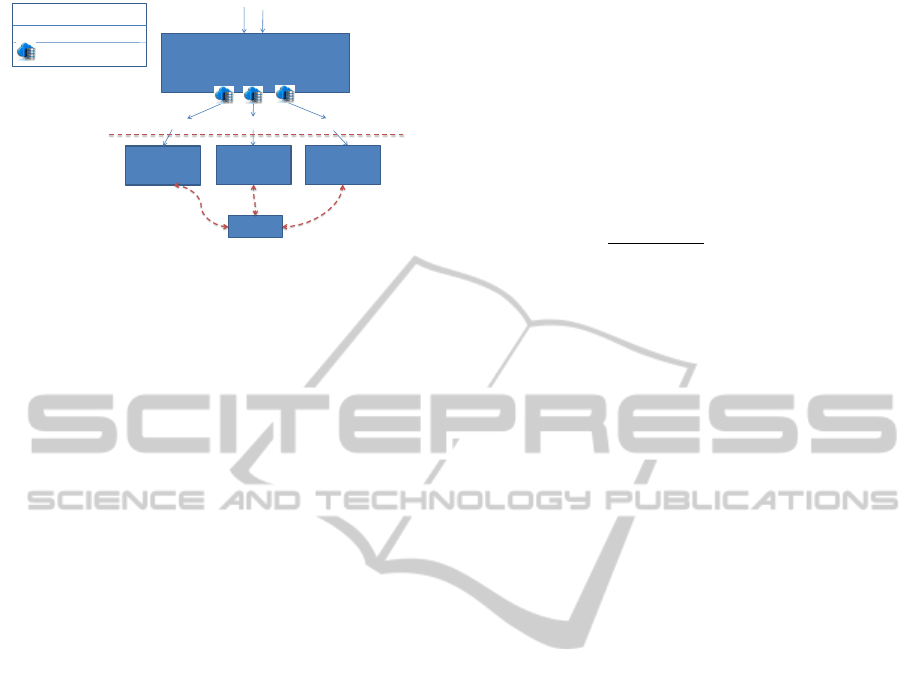
Figure 4 demonstrates D-DF’s architecture. D-DF

is divided into two phases:

• Initialization phase: a certain number of edit paths

is generated using A*-GED. Moreover, a ﬁrst up-

per bound (UB-best) is computed using a bipartite

graph matching (BP). The interested reader is re-

ferred to (Riesen, 2009) for more details.

• Distributed phase: each worker on the map side

takes an edit path to be solved using DF-GED.

When a map worker m

succeeds in ﬁnding a bet-

ter upper bound, it updates the value of UB-best

and notiﬁes the other map workers so that they

get the new value. Also, when a worker is done

with one edit path, it communicates with the mas-

ter program in order to get another edit path that

has not been explored yet. This job ﬁnishes when

there is no more edipath to explore. The value

UB-best represents the optimal solution (i.e., dis-

tance) between g

and g

ICPRAM2015-DoctoralConsortium

Initialization:

Generate X edit paths using A*-GED

Compute a first upper bound UB-best

DF-GED with

UB-best

g2 g1

𝑃𝐸𝑃

𝑋

PEP

UB-best

Partial Edit Path

Global upper bound

Save to hadoophard disk

DF-GED with

UB-best

DF-GED with

UB-best

• Update UB-best if a better value is found

• Notifiy other workers so that they can get

the new value

Update &

notify ?

Update &

notify ?

Update &

notify ?

Figure 4: The architecture of DF-F.

6 EXPERIMENTS

6.1 Environment

Evaluations are conducted on a 4-core Intel i7 proces-

sor 3.07GHz and 8 GB of memory.

6.2 Protocol and Quality Measures

In this section, we explain the protocol used to

evaluate the two sequential and optimal approaches

(A*GED and DF-GED). This Protocol is three-fold:

• Calculating the distance matrix under a small time

constraint.

• Calculating the distance matrix under a big time

constraint.

• Classiﬁcation test under a reasonable time con-

straint.

Let S be a graph dataset consisting of m graphs,

S = {g

, g

, ..., g

}. Let P = {A*GED, DF-GED}

be the set the compared methods. Given a method

p ∈ P , we computed the square distance matrix

∈ M

), that holds every pairwise compar-

ison M

i, j

= d

, g

), where the distance d

, g

)

is the value returned by the method p on the graph

pair (g

, g

) within a certain time and memory limits.

Hence, M

A*GED

and M

DF-GED

denote distance matri-

ces of A*GED and DF-GED methods, respectively.

Let GT ∈ M

) be the reference matrix that

holds the best found distance for each pair of graphs.

We aim at comparing the errors committed by the dif-

ferent methods as well as their speed under a time

constraint C

and a memory constraint C

when

graphs sizes increase (i.e., on GRECk) and also on

GREC-mix. To this objective, we test the accuracy of

P when C

is small (C

= 350ms) and when C

is big

= 5 minutes). C

is set to 1GB during all the ex-

periments. We expect A*GED to violate C

specially

when graphs get larger.

In the following, we deﬁne the measurements used

for evaluating our protocol:

Deviation. we evaluate the error committed by a

method p over the reference distances. To this end,

we measure an indicator called deviation and deﬁned

by the following equation:

deviation(i, j)

i, j

− GT

i, j

, ∀(i, j) ∈ J1, mK

, ∀p ∈ P

(2)

Where GT

i, j

is the smallest distance among all dis-

tances generated by P when matching g

and g

Running Time. we measure the running time

in millisecond for each comparison d(g

). This

value reﬂects the overall time for GED computation

including all the inherits costs computations (i.e.,

g(p); h(p); and U B)

For the classiﬁcation test, we are interested in the

average computation time (t) which corresponds to

the average time elapsed when classifying all the test

graphs of GREC and the classiﬁcation accuracy (AC)

which deﬁnes the error made when classifying the test

graphs of GREC. Both measurements are achieved

when C

= 500ms and C

= 1GB. The classiﬁcation

stage is performed by a 1-NN classiﬁer. Each test

graph g

is compared to the entire training set. The

nearest neighbor’s label is assigned to g

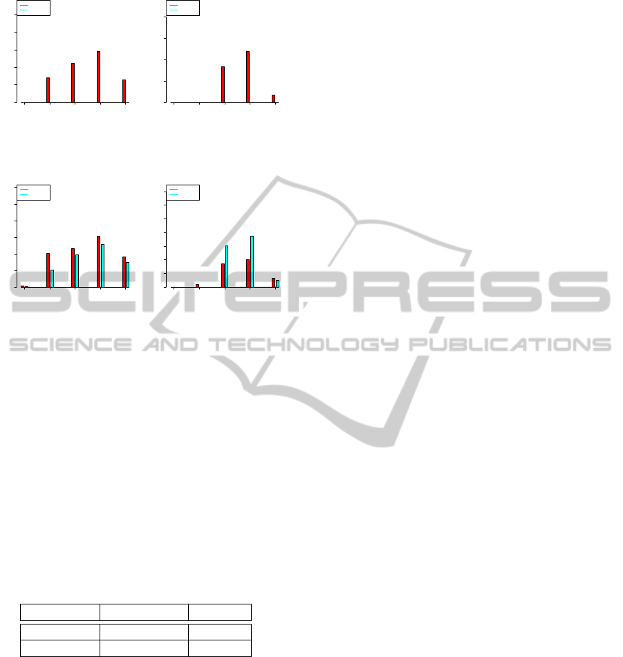
7 RESULTS AND DISCUSSION

Figure 5 shows the deviation results under 350 mil-

liseconds and 5 minutes respectively. We observe that

DF-GED always outperforms A*GED under the same

time constraint. For all GED computations, DF-GED

gives the best distance (i.e., GT

i, j

) and so its deviation

is always 0%. In contrast with DF-GED, the deviation

of A*GED decreases when C

= 5 minutes. How-

ever, when the size of graphs increase (e.g., GREC15

and GREC20), the deviation starts to converge due to

memory saturation where the best recently known so-

lution is outputted before halting.

Figure 6 demonstrates the running time of both

A*GED and DF-GED. When C

= 350 milliseconds

both running times are relatively equal on GREC15

and GREC20 and that is because non of them is

able to ﬁnd an optimal solution before exceeding C

When C

increases, DF-GED becomes faster as it ex-

plores the search tree in a depth-ﬁrst way (i.e., not

stopped by C

) while pruning the search tree thanks

to its upper and lower bounds as well as the prepro-

cessing step, see Section 4.3. On the other hand,

DistributedGraphMatchingandGraphIndexingApproaches-ApplicationstoPatternRecognition

GREC5 GREC10 GREC15 GREC20 GREC−mix

Number of vertices

Mean deviation in (%)

0 20 40 60 80 100

A*GED

DF−GED

GREC5 GREC10 GREC15 GREC20 GREC−mix

Number of vertices

Mean deviation in (%)

0 20 40 60 80

A*GED

DF−GED

Figure 5: Deviation. Left:(350 milliseconds), Right:(5 min-

utes).

GREC5 GREC10 GREC15 GREC20 GREC−mix

Number of vertices

Mean running time in milliseconds

0 100 200 300 400 500 600

A*GED

DF−GED

GREC5 GREC10 GREC15 GREC20 GREC−mix

Number of vertices

Mean running time in milliseconds

0 50000 150000 250000 350000

A*GED

DF−GED

Figure 6: Running Time. Left:(350 milliseconds), Right:(5

minutes).

A*GED does not continue for further exploration on

GREC15 and GREC20 because of the size of the in-

volved graphs where available memory is exhausted

and so the best recently known solution is given be-

fore halting.

For the classiﬁcation experiment, 151008 compar-

isons are performed on 286 training graphs and 528

test graphs of the GREC dataset. As depicted in Ta-

ble 1, results show that the classiﬁcation accuracy AC

of DF-GED is 2.3 times higher under the same C

where C

=500 milliseconds. Moreover, DF-GED is

1.7 times faster as the average time t is smaller.

Table 1: Classifying graphs of GREC (C

= 500 millisec-

onds).

Algorithms t AC

A*GED 119491.5 ms 42.23%

DF-GED 69006.3 ms 98.48 %

8 CONCLUSION AND

PERSPECTIVES

As presented in this report, we have discussed the ﬁrst

part of the thesis, we have considered the problem

of GED computation for PR. Graph edit distance is

a powerful and ﬂexible paradigm that has been used

in different applications in PR. The exact algorithm,

A*GED, presented in the literature suffers from high

memory consumption and thus cannot match large

graphs due to the exponential complexity of GED

computation. In this report, we proposed another ex-

act GED algorithm, DF-GED, which is based on a

depth-ﬁrst tree search. This algorithm speeds up the

computations of graph edit distance thanks to its up-

per and lower bounds pruning strategy and its prepro-

cessing step. Moreover, this algorithm does not ex-

haust memory as the number of pending edit paths

that are stored in the set OPEN is relatively small

thanks to the depth-ﬁrst search where the number of

pending nodes is |V 1|.|V 2| in the worst case.

In the experimental section, we have proposed to

evaluate sub-optimally both exact methods: A*GED

and DF-GED under some memory and time con-

straints. Experiments on the GREC database em-

pirically demonstrated that DF-GED outperforms

A*GED in terms of accuracy, speed and classiﬁcation

rate. For future work, we aim at measuring the qual-

ity of solutions found by our distributed approach (D-

DF) as well as the aforementioned approximate meth-

ods. All these different graph edit distance computa-

tions will be evaluated on different PR databases. We

expect D-DF to outperform other methods in terms of

accuracy. We also want to conduct a scalability study

to show the importance of such a ﬂexible distributed

approach for solving PR problems.

In the next phase of the thesis, we also aim

at proposing a distributed graph-indexing approach

where a graph g is fragmented and indexed in a fully

distributed manner.

REFERENCES

(1998). A genetic algorithm and its parallelization for graph

matching with similarity measures. 2(2):68–73.

A.D.J. Cross, R. W. and Hancock, E. (1997). Inexact graph

matching using genetic search. Pattern Recognition,

pages 953–970.

Allen, R., C. L. M. S. T. S. S. L. and Yasuda, D. (1997). A

parallel algorithm for graph matching and its maspar

implementation. Pattern Recognition, page 490501.

Andreas Fischer, Ching Y. Suen, V. F. K. R. H. B. (2013). A

fast matching algorithm for graph-based handwriting

recognition. GbRPR 2013, pages 194–203.

Andrew D. J. Cross, E. R. H. (1998). Graph matching with

a dual-step em algorithm. IEEE Trans. Pattern Anal.

Mach. Intell., 20:1236–1253.

Bunke, H. (1983). Inexact graph matching for struc-

tural pattern recognition. Pattern Recognition Letters,

1(4):245–253.

Combier, C., Damiand, G., and C., S. (2013). Map edit

distance vs graph edit distance for matching images.

In Proc. of 9th Workshop on Graph-Based Represen-

tation in Pattern Recognition (GBR), volume 7877,

pages 152–161.

ICPRAM2015-DoctoralConsortium

Conte, D., Foggia, P., Sansone, C., and Vento, M. (2004).

Thirty Years of Graph Matching. 18(3):265–298.

Cormen, T. H., Leiserson, C. E., Rivest, R. L., and Stein,

C. (2009). Introduction to Algorithms, Third Edition.

The MIT Press, 3rd edition.

Dean, J., G. S. (2004). Mapreduce : Simpliﬁed data pro-

cessing on large clusters. Symposium on Operating

Systems Design and Implementation., 28:137149.

Fankhauser, S., Riesen, K., Bunke, H., and Dickinson, P. J.

(2012). Suboptimal graph isomorphism using bipar-

tite matching. IJPRAI, 26.

Finch, Wilson, e. a. (1998). An energy function and contin-

uous edit process for graph matching. Neural Compu-

tat, 10.

Justice, D. and Hero, A. (2006). A binary linear program-

ming formulation of the graph edit distance. IEEE

Transactions on Pattern Analysis and Machine Intel-

ligence, 28(8):1200–1214.

Kollias, G. (2012). Fast parallel algorithms for graph simi-

larity and matching.

Kuner, P. and Ueberreiter, B. (1988). Pattern recognition

by graph matching: Combinatorial versus continuous

optimization. International Journal in Pattern Recog-

nition and Artiﬁcial Intelligence, 2:527542.

M. Neuhaus, K. R. and Bunke., H. (2006). Fast suboptimal

algorithms for the computation of graph edit distance.

Proceedings of 11th International Workshop on Struc-

tural and Syntactic Pattern Recognition., 28:163172.

Patwary, M. M. A., Bisseling, R. H., and Manne, F. (2010).

Parallel greedy graph matching using an edge parti-

tioning approach. Proceedings of the fourth interna-

tional workshop on High-level parallel programming

and applications - HLPP ’10, page 45.

Plantenga, T. (2013). Inexact subgraph isomorphism in

mapreduce. Journal of Parallel and Distributed Com-

puting, page 164175.

Qiu, H. and Hancock, E. R. (2006). Graph matching and

clustering using spectral partitions. Pattern Recogni-

tion, 39(1):22–34.

Riesen, K., B. H. (2009). Approximate graph edit distance

computation by means of bipartite graph matching.

Image and Vision Computing., 28:950959.

Riesen, K., Fankhauser, S., and Bunke, H. (2007). Speed-

ing up graph edit distance computation with a bipartite

heuristic. In MLG.

Sanfeliu, A. and Fu, K. (1983). A distance measure be-

tween attributed relational graphs for pattern recogni-

tion. IEEE Transactions on Systems, Man, and Cyber-

netics, 13:353–362.

Tsai, W.-H. and Fu, K.-S. (1979). Error-correcting isomor-

phisms of attributed relational graphs for pattern anal-

ysis. Systems, Man and Cybernetics, IEEE Transac-

tions on, 9(12):757–768.

Tsai, W. H. and Fu, K. S. (1983). IEEE Transactions on

Systems, Man and Cybernetics, pages 48–62.

Vento, M. (2014). A long trip in the charming world of

graphs for pattern recognition. Pattern Recognition.

W. Christmas, J. K. and Petrou., M. (1995). Structural

matching in computer vision using probabilistic relax-

ation. IEEE Trans. PAMI,, 2:749764.

Zeng, Z., Tung, A. K. H., Wang, J., Feng, J., and Zhou,

L. (2009). Comparing stars: On approximating graph

edit distance.

DistributedGraphMatchingandGraphIndexingApproaches-ApplicationstoPatternRecognition