
Range and Vision Sensors Fusion for Outdoor 3D Reconstruction
Ghina El Natour
1
, Omar Ait Aider
1
, Raphael Rouveure
2
, Franc¸ois Berry
1
and Patrice Faure
2
1
Blaise Pascal Institut UBP-CNRS 6602, Blaise Pascal University, Clermont-Ferrand, France
2
IRSTEA, Institut national de Recherche en Sciences et Technologies pour l’Environnement et l’Agriculture,
Clermont-Ferrand, France
Keywords:
3D Reconstruction, Multi-sensor Calibration, Range Sensor, Vision Sensor.
Abstract:
The conscience of the surrounding environment is inevitable task for several applications such as mapping,
autonomous navigation and localization. In this paper we are interested by exploiting the complementarity
of a panoramic microwave radar and a monocular camera for 3D reconstruction of large scale environments.
Considering the robustness to environmental conditions and depth detection ability of the radar on one hand,
and the high spatial resolution of a vision sensor on the other hand, makes these tow sensors well adapted for
large scale outdoor cartography. Firstly, the system model of the two sensors is represented and a new 3D
reconstruction method based on sensors geometry is introduced. Secondly, we address the global calibration
problem which consists in finding the exact transformation between radar and camera coordinate systems.
The method is based on the optimization of a non-linear criterion obtained from a set of radar-to-image target
correspondences. Both methods have been validated with synthetic and real data.
1 INTRODUCTION
Virtual world creation and the conscience of real
world are important tasks for several applications
such as mapping, autonomous navigation and local-
ization. Therefore, data acquisition through a sensor
or a host of sensors is required. Despite the large
number of studies and researches in this field ((Bha-
gawati, 2000; Kordelas et al., 2010)), there are still
many challenges for fully automatic and real time
modeling process together with high quality results,
because of acquisition and matching constraints, call-
ing for more contributions. The methods can be clas-
sified according to sensors used: vision sensor, range
sensor, odometers or a set of sensors. To overcome
the limitations of single sensor approaches, multi-
sensory fusion have been recently a point of interest
in widespread applications and researches especially
for 3D mapping applications.
Regarding the low cost and high spatial resolution
of vision sensors, a huge number of vision based ap-
proaches for 3D reconstruction have been proposed.
For example, a method based on a single panoramic
image was described in Sturm et al. (Sturm, 2000).
Gallup et al. (Gallup et al., 2007) worked on frames of
a single video-camera to reconstruct the depth maps.
Some other examples can be found in (Pollefeys et al.,
2008) and (Royer et al., 2007). Methods for 3D
scene reconstruction from an image sequence can be
grouped in two classes: Structure-from-Motion and
dense stereo. In the last years, many works tend to
fill the gap between the two approaches in order to
propose methods which may handle very large scale
outdoor scenes. Results seem to be of good quality
though it recommends a large amount of input data
and heavy algorithms which make it not quite suit-
able for real time processing. It is also known that
techniques for large scene reconstruction by vision
generally suffer from scale factor drift and loop clos-
ing problems. In addition, vision sensors present sev-
eral drawbacks due to the influence of image quality
when illumination and weather conditions are dete-
riorated. For this reason, tapping into active sensors
has become essential. Furthermore, the capability of
range sensors to work in difficult atmospheric condi-
tions and its decreasing cost, made it well suited for
extended outdoor robotic applications. For example,
Grimes et al. (Grimes and Jones, 1974) investigated
on automotive radar and discussed in detail its config-
urations and different potential applications for vehi-
cles. In (Rouveure et al., 2009), RAdio Detection And
Ranging (RADAR) is used for simultaneous localiza-
tion and mapping (R-SLAM algorithm) applications
in agriculture. In (Austin et al., 2011), single radar is
used to reconstruct sparse 3D model. However, range
sensors fail to recognize elevation, shape, texture, and
202
El Natour G., Ait Aider O., Rouveure R., Berry F. and Faure P..
Range and Vision Sensors Fusion for Outdoor 3D Reconstruction.
DOI: 10.5220/0005324302020208
In Proceedings of the 10th International Conference on Computer Vision Theory and Applications (VISAPP-2015), pages 202-208
ISBN: 978-989-758-089-5
Copyright
c
2015 SCITEPRESS (Science and Technology Publications, Lda.)

size of a target. Many solutions based on the com-
bination of depth and vision sensors are described in
the literature. An example of this fusion can be found
in (Forlani et al., 2006), an automatic classification of
raw data from LIght Detection And Ranging (LIDAR)
in external environments, and a reconstruction of 3D
models of buildings is presented. The Lidar provides
a large number of 3D points which requires data pro-
cessing algorithms, and can be memory and time con-
suming. SLAM applications with Kinect are also nu-
merous ((Smisek et al., 2013; Schindhelm, 2012; Pan-
cham et al., 2011)). Yet the performances are gener-
ally limited in outdoor environment due to the small
depth range and sensitivity to illumination conditions.
In this paper, we are investigating the combination
of panoramic MMW (Millimetre Waves) radar and a
camera in order to achieve a sparse 3D reconstruc-
tion of large scale outdoor environments. Recently,
this type of fusion has been studied for on-road obsta-
cle detection and vehicle tracking: in (Bertozzi et al.,
2008), camera and radar were integrated with an in-
ertial sensor to perform road obstacle detection and
classification. Other works on radar-vision fusion for
obstacle detection can also be found in literature (see
for example (Roy et al., 2009; Hofmann et al., 2003;
Wang et al., 2011; Haselhoff et al., 2007; Alessan-
dretti et al., 2007; Bombini et al., 2006)). However,
we are not aware of any work using radar and camera
for outdoor 3D reconstruction. More than data fusion,
our aim is to build a 3D sensor which provides tex-
tured elevation maps. Therefore, a geometrical model
of the sensors and a calibration technique should be
provided. These two sensors are complementary: we
rely on the fact that the distance from an object to the
system is given by the radar measurements having a
constant range error with increasing distance. While
its altitude and size can readily be extracted from the
image. The camera/radar system is rigidly fixed and
the acquisitions from the two sensors are done simul-
taneously. In multi-sensors systems, each sensor per-
forms measurements in its own coordinate system.
Thus, one needs to transform these measurements into
a global coordinate system. Our goal is to simplify
this tricky and important step, which is crucial for the
matching process and inhibits the reconstruction ac-
curacy so that it can be carried out easily and any-
where, by a non-expert operator. Therefore we pro-
pose a technique which uses only a set of radar-to-
image point matches. These points are simple targets
positioned in front of the camera/radar system and the
distances between them are measured. A nonlinear
geometrical constraint is derived from each match and
a cost function is built. Finally, the transformation be-
tween the radar and the camera frames is recovered
by a LM-based optimization (Levenberg-Marquardt).
Once the calibration parameters are defined, the 3D
reconstruction of any radar-vision matched target can
be achieved resolving a system of geometrical equa-
tions. Indeed, the intersection point of a sphere cen-
tered on radar frame origin and a light ray passing
through the camera optical center is the 3D position
of the object. So, a small amount of input data (single
image and panoramic frame) is sufficient to achieve
a sparse 3D map allowing thereby the real time pro-
cessing.
The paper is organized as follows: In section 2 we
describe the camera and radar geometrical models and
we addressed the 3D reconstruction problem. Section
3 focuses on the calibration method. And finally, ex-
perimental results obtained with both synthetic and
real data are presented and discussed in section 4.
2 3D RECONSTRUCTION
3D reconstruction of large scale environment is a
challenging topic. Our goal is to build a simple 3D
sensor which provides textured elevation maps as il-
lustrated in fig.1. In order to achieve the 3D recon-
struction a preliminary steps must be carried on: Data
acquisition should be done simultaneously by each of
the sensors having an overlapping field of view. Fea-
tures extraction and matching between the data pro-
vided by these two sensors is a difficult process since
it is inherently different and thus it cannot be easily
compared or matched. For the current stage, further
works are under progress for this step. Finally, the
calibration consists of determining the transformation
mapping targets coordinates from one sensor frame to
another.
Figure 1: An illustration of elevation map generation ex-
ploiting radar and vision complementarity.
2.1 The System Model
The system model is formed by a camera and radar
rigidly linked. The camera frame and centre are de-
RangeandVisionSensorsFusionforOutdoor3DReconstruction
203

Figure 2: System geometry: R
c
and R
r
are the camera and
radar frames respectively. Polar coordinates m
r
(α,r) of the
target are provided by radar data but not the elevation angle.
The Light ray L and the projected point p in the image I
c
are
shown together with the horizontal radar plane.
noted R
c
and O
c
(x
O
c
,y
O
c
,z
O
c
) respectively. Similarly
R
r
and O
r
(x
O
r
,y
O
r
,z
O
r
) are respectively the radar’s
frame and centre. The sensors system is illustrated in
fig.2. The radar performs acquisitions over 360
◦
per
second thanks to its 1
◦
step rotating antenna. It gener-
ates each second a panoramic image of type PPI (Plan
Position Indicator), where detected targets are local-
ized in 2D polar coordinates. The radar-target dis-
tance measurement is based on the FMCW principle
(Skolnik, 2001). It can be shown that the frequency
difference (called beat frequency) between the trans-
mitted signal and the signal received from a target is
proportional to the sought distance. The reflected sig-
nal has a different frequency because of the continu-
ous variation of the transmitted signal around a fixed
reference frequency. Therefore, the radar performs
a circular projection on a horizontal plane passing
through the centre of the antenna first lobe, the pro-
jected point is denoted m
r
(α,r). So, the real depth r
and azimuth α of a detected target is provided without
any altitude information. For the camera, we assume
a pinhole model consisting of two transformations:
first transformation projects a 3D point
e
M(x, y,z, 1)
T
into
e
p(u,v,1)
T
(in homogeneous coordinates system)
of the image plane Ic and it is written as follows:
w
e
p = [K|0]I
4×4
e
M (1)
w
u
v
1
=
f
x
0 u
0
|0
0 f
y
v
0
|0
0 0 1 |0
1 0 0 0
0 1 0 0
0 0 1 0
0 0 0 1
x
y
z
1
(2)
Where w is a scale factor and K is the matrix of in-
trinsic parameters, assumed to be known, since the
camera is calibrated (Bouguet, 2004). One can write:
e
M =
K
−1
w
e
p
1
=
wm
1
(3)
and
m = K
−1
e
p =
m
1
m
2
m
3
T
(4)
Second, the calibration parameters are described by a
3D transformation (rotation R and translation t) map-
ping any point
e
M from the camera frame R
c
to a point
e
Q(X,Y,Z, 1)
T
in the radar frame R
r
such as:
e
M = A
e
Q (5)
with A the extrinsic matrix parameters.
A =
R t
0 1
=
R11 R12 R13 tx
R21 R22 R23 ty
R31 R32 R33 tz
0 0 0 1
(6)
Replacing
e
M in equation (1) by the formula in (5),
provides the final transformation mapping 3D to 2D
point as follows:
w
e
p = [K|0]A
e
Q (7)
2.2 The 3D Reconstruction Method
Because of the projected geometry of vision and radar
sensors, part of informations are lost while acquisi-
tion. 3D reconstruction of an unknown scene is then
the compensation of missing data from two dimen-
sions acquisitions. In order to recover the third dimen-
sion we proceed as follows: a 3D point Q detected by
both camera and radar is the intersection of the light
ray L passing by the optical centre and the sphere C
centred on radar as shown in fig.3. Therefore, its 3D
coordinates are obtained by estimating the intersec-
tion point Q is lying on the sphere C whose equation
is:
(C) (x −x
O
r
)
2
+ (y −y
O
r
)
2
+ (z −z
O
r
)
2
= r
2
(8)
Our method consists of three steps: First the scale fac-
tor w is computed. From equation (3), x, y and z can
be written as a function of w: x = wm
1
, y = wm
2
and
z = wm
3
, thereby, leading to a quadratic equation in
w:
w
2
(m
2
1
+ m
2
2
+ m
2
3
) −2w(m
1
x
O
r
+ m
2
y
O
r
+ m
3
z
O
r
)
+(x
2
O
r
+ y
2
O
r
+ z
2
O
r
−r
2
) = 0 (9)
Figure 3: Q is the intersection of light ray L and the sphere
C at α. m
r
is the projected 2D radar point and V P is the
vertical plane of the target at α.
VISAPP2015-InternationalConferenceonComputerVisionTheoryandApplications
204

Since we are working in large scale environment,
the targets are usually too far compared to the base-
line (the distance between the radar and camera
frames). Then, the camera is always inside the sphere
C, so theoretically, two solutions exist, w and w
0
.
From these solutions, two points
e
M(x, y,z, 1)
T
and
f
M
0
(x
0
,y
0
,z
0
,1)
T
relative to the vision sensor are de-
duced from (20). Secondly, the transformation is ap-
plied to these latter in order to determine their coor-
dinates in the radar frame system. The two points in
radar frame are then:
e
Q = A
−1
e
M and
e
Q
0
= A
−1
f
M
0
(10)
Finally, azimuth of these 3D points are computed
from the Cartesian coordinates. Thereby, the correct
solution is selected by comparing the computed az-
imuth angle and the one measured by the radar. The
calibration step is then requisite in order to determine
the transformation matrix A.
3 SYSTEM CALIBRATION
The calibration stage is an important factor affecting
the reconstruction accuracy. Hence, it is required to
develop an accurate calibration method. For sum ap-
plication one might need to recalibrate the system due
to mechanical vibrations or to enable free positioning
of the sensors thus it should be rather simple to im-
plement.
3.1 Related Work
The closest work on camera-radar system calibra-
tion is the work of S.SUGIMOTO et al. (Sugimoto
et al., 2004). Radar’s acquisitions are considered to
be coplanar, since it perform a planar projection on its
a horizontal plane. Therefore, the transformation A is
a homography H between image and radar planes. In
spite of its theoretical simplicity, this method is hard
to be implemented. Indeed, while the canonical target
is being continuously moved up and down by a me-
chanical system, it should be simultaneously acquired
by radar and camera. Then, pairs of matches (4 pairs
at least) corresponding to the exact intersection of the
target with the horizontal plane of the radar, are ex-
tracted. Moreover, due to sampling frequency, the ex-
act positions are determined from the maximum of the
intensity reflected by the target using bilinear interpo-
lation of the measurement samples along the vertical
trajectory of each target.
3.2 The Proposed Calibration Method
Our goal is to determine rotation and translation. The
only constraint for the proposed method is the a priori
knowledge of distances between the targets used for
calibration. For an azimuth angle α, we have the nor-
mal to the plane V P, ~n = (sin(α),−cos(α), 0). Since
V P is a vertical plane passing by O
r
it have the fol-
lowing equation:
X sin(α) −Y cos(α) = 0
(11)
O
r
(x
r
,y
r
,z
r
) and r are the sphere centre and radius
respectively in radar coordinate frame. The sphere C
is then centred on O
r
(0,0, 0), equation (9) becomes:
(C)(X)
2
+ (Y )
2
+ (Z)
2
= r
2
(12)
From equation (7), X, Y and Z are expressed in terms
of unknown A and w:
X = A
−1
11
wm
1
+ A
−1
12
wm
2
+ A
−1
13
wm
3
+ A
−1
14
Y = A
−1
21
wm
1
+ A
−1
22
wm
2
+ A
−1
23
wm
3
+ A
−1
24
Z = A
−1
31
wm
1
+ A
−1
32
wm
2
+ A
−1
33
wm
3
+ A
−1
34
(13)
For n matches, system (S
1
) is obtained, with i = 1 →n
and ε the residuals:
(S
1
)
X
2
i
+Y
2
i
+ Z
2
i
−r
2
i
= ε
i
1
X
i
sin(α
i
) −Y
i
cos(α
i
) = ε
i
2
The equations are expressed with respect to a param-
eter vector [γ
x
,γ
y
,γ
z
,t
x
,t
y
,t
z
,w
i
], γ are the three rota-
tional angles relative to Ox, Oy and Oz. In order to
calculate the scale factor w
i
, we applied the general-
ized form of the Pythagorean theorem for an unspeci-
fied triangle, to the triangle formed by two 3D points
M
1
, M
2
with O
c
as illustrated in fig.4. This gives the
following equations:
Figure 4: The triangle formed by M1, M2 (3D points in the
camera frame) and O
c
is shown. d
12
is the known distance
between M1 and M2 and D
1
, D
2
are their depths relative to
O
c
.
D
2
1
+ D
2
2
−2L
12
= d
2
12
(14)
where
L
12
= D
1
D
2
cos(θ
12
) (15)
D
i
is the depth of the point relative to O
c
and it is re-
lated to the scale factor w
i
, and the angle β
i
formed
between the principle point p
c
and pixel p
i
by the for-
mula:
D
i
=
w
i
cos(β
i
)
(16)
with
cos(β
i
) =
p
T
c
(KK
T
)
−1
p
i
√
(p
T
c
(KK
T
)
−1
p
c
)(p
T
i
(KK
T
)
−1
p
i
)
(17)
RangeandVisionSensorsFusionforOutdoor3DReconstruction
205
d
i j
is the known distance between points and θ
i j
is the
angle between two rays lining up the 3D points with
O
c
. Since we have six degrees of freedom (DOF):
three for rotation angles and three for the translation,
both relative to Ox, Oy and Oz, we need at least six
points. With six 3D points, we have 15 inter-distances
so we obtain a system (S
2
) of 15 equations in terms
of w
i=1→6
and ε are the residuals:
(S
2
)
n
D
2
i
+ D
2
j
−2L
i j
−d
2
i j
= ε
i j
3
The system is solved by the algorithm of
Levenberg-Marquardt, based on non-linear least
squares optimization of the sum of squared residuals
(ε)
2
, in order to determine the approximate solution
as shown hereafter:
∑
(ε
i
1
)
2
+ (ε
i
2
)
2
and
∑
(ε
i j
3
)
2
(18)
4 RESULTS
4.1 Simulation Results
Simulations with synthetic data were carried out in
order to test the efficiency and the robustness of the
new methods with respect to numerous parameters
such as number of points and noise level. Sets of
3D points are randomly generated following a uni-
form random distribution within a cubic work space
in front of the camera-radar system. The projected
pixel of each 3D point is computed using the pinhole
model of the camera, and its spherical coordinates are
computed. At first, both algorithms were tested with-
out additional noise and a very low error levels were
obtained ( 1.180 10
−6
m on translation, 1.269 10
−12
◦
on rotation and 3.671 10
−14
m on reconstruction re-
sults). Afterwards, the simulations were extended em-
ulating realistic cases, in order to test the accuracy of
the calibration and reconstruction methods. Therefore
synthetic data are perturbed by uniformly distributed,
random noise. Linear increasing of noise level is ap-
plied on data, starting from level 1 corresponding to
±0.5 pixels, ±0.5
◦
on azimuth angle, ±0.5cm on dis-
tance up to level 25 corresponding to ±2.5 pixels,
±5
◦
on azimuth angle, ±50cm on distance and ±5mm
on inter-distance. This multi level noise is added pro-
gressively on data. Both calibration and reconstruc-
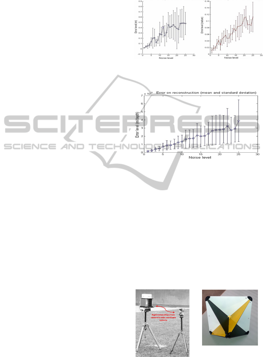
tion errors graphs are shown in fig.5 and 6.
The number of matches used for the calibration
process is 10. It should be noticed that the increasing
noise on the rotation and translation increases the er-
rors: non-linear algorithms are affected by noise and
yet our algorithm shows an acceptable behaviour in
the presence of noisy data. The graph in fig.6 shows
Figure 5: Calibration error with respect to the noise level.
Left: translation error in meter. Right: rotation error in
radian. The graphs show the mean and the standard devia-
tion of RMSE upon 6 specimen.
Figure 6: Reconstruction error with respect to the noise
level. The error is in meter relative to the points depths
(r). The mean and standard deviation over 50 reconstructed
points are shown.
the mean and standard deviation of the RMSE upon
50 reconstructed points. Despite of the slight raising
of error with increasing noise level, it is quite clear
that the method is very robust in the presence of a re-
alistic noise level.
4.2 Experimental Results
The radar and the camera were mounted in a fixed
configuration in order to carry out real data acquisi-
tions (for the current stage the radar antenna rotates
360
◦
but the camera is stable ). The system is shown
in fig.7. The radar is called K2Pi. It has been devel-
Figure 7: Radar and cam-
era system.
Figure 8: The canonical
targets were painted in or-
der to readily extract the
centre (yellow cross).
VISAPP2015-InternationalConferenceonComputerVisionTheoryandApplications
206
oped by Irstea Institute. The optic sensor used is uEye
by IDS (Imaging Development Systems). Camera
and radar’s characteristics are listed in table 1. Eight
canonical targets were placed in front of the sensors
system. Metallic targets are highly reflective. Their
tetrahedral and spheric forms provide the same radar
waves reflection regardless of their position relative to
the radar. The depth of targets is chosen to be slightly
close (between 6 and 14m) and targets were painted
to increase the contrast and thus facilitate the features
(targets centres) extraction from the image. The fig.8
shows an example of these targets. First the system
is calibrated using our algorithm. The inter-distances
between the targets centres are measured precisely,
and an image and a panoramic of the 8 targets in ran-
dom configurations are used. image and radar targets
are extracted and matched manually.
Table 1: Camera and radar characteristics.
Camera characteristics
Sensor technology CMOS
Sensor size 4.512 ×2.880mm
Pixel size 0.006mm
Resolution (h ×v) 752 ×480
Focal distance 8mm
Radar characteristics
Carrier frequency 24GHz
Antenna gain 20dB
Range 3 −100m
Angular resolution 4
◦
Distance resolution 1m
Distance precision 0.02m
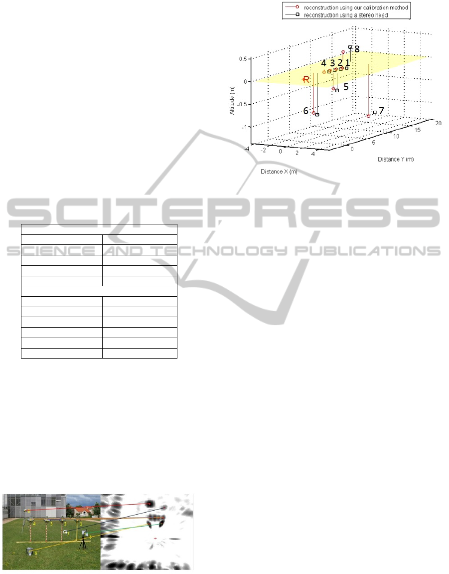
Fig.9 shows the corresponding pixels and radar
points extracted in the image of the camera and the
panoramic image. In order to validate the recon-
struction method and to assess our calibration re-
sults, the 8 targets were placed at different heights
and depths. The matches were also extracted and the
reconstruction is done in radar frame. Fig.10 repre-
sent the results of the reconstruction technique, using
the method of section 3.2 and reconstruction from a
stereo head, used as ground truth. The ground truth
point set and the reconstructed one were registered us-
Figure 9: An image and a panoramic of targets. The targets
are numbered from 1 to 8: one Luneburg lens and seven
trihedral corners. The yellow crosses indicate the centres of
the targets. Manually extracted matches between the image
and the PPI are shown.
Figure 10: The reconstruction results using results from
both, our reconstruction methods (circular points) and the
stereo head method as a ground truth (squared points).
Radar position is notified by the letter R.
ing ICP (Iterative Closest Point) algorithm. The RMS
of the reconstruction error is about 0.1939m with a
standard deviation of 0.015m. The results show a re-
alistic error for the 3D reconstruction of targets at a
mean depth of 12m.
A qualitative evaluation of the reconstruction
method is also provided in fig.11. In this exemple, an
interactive segmentation and matching of the data are
done. An accurate result of a 3D reconstruction of a
real urban scene is shown and inhanced with a texture
map. In fact, the interest of this sensor fusion is shown
in this example as the radar provides no information
about the elevation of the bridge, so it is detected as a
barrier which is corrected after the reconstruction.
5 CONCLUSIONS
In this paper, we presented a 3D reconstruction
method using a radar and a camera for extended out-
door applications and a geometrical algorithm for spa-
tial calibration. Our methods are both validated by
simulated data, and real experiments with sparse data.
Results show the accuracy of these methods and prove
the interest of the application of these two sensors for
3D reconstruction of outdoor scenes and quite a good
behavior in the presence of noise. To our knowledge,
these types of sensors have not been used for large
outdoor reconstruction applications. For the current
stage, sparse point matches are extracted manually,
therefore, RANSAC-like algorithms must be settled
up to make automatic matching and to achieve dense
3D reconstruction. Further real time reconstruction
experiments of urban scenes should be carried out.
RangeandVisionSensorsFusionforOutdoor3DReconstruction
207
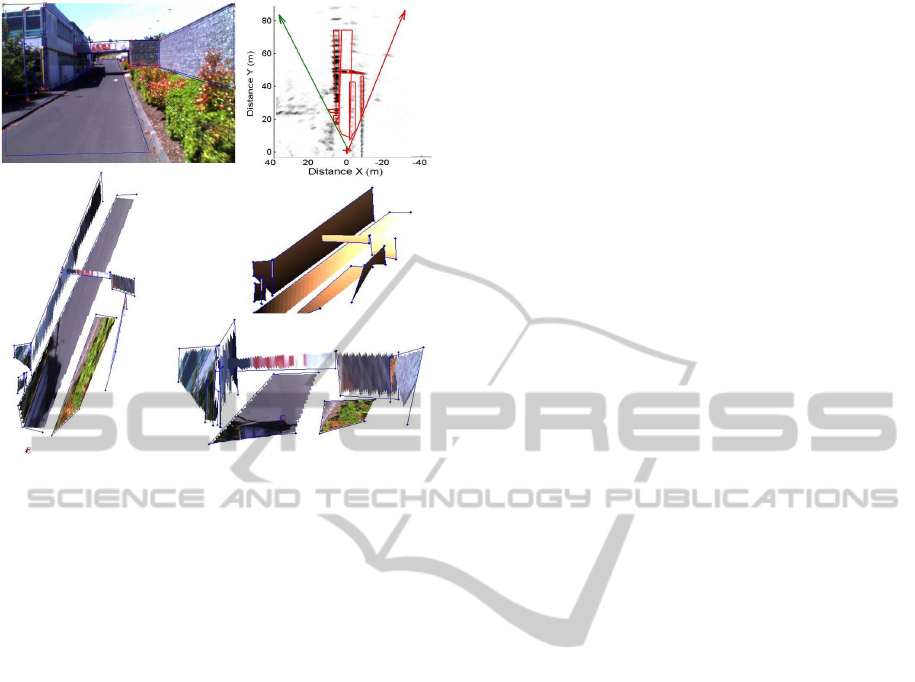
Figure 11: 3D reconstructed urban scene. Top line: seg-
mented image and panoramic data. Right middle: the 3D
reconstruction results. Right bottom and left bottom: two
different views of textured 3D reconstruction results.
REFERENCES
Alessandretti, G., Broggi, A., and Cerri, P. (2007). Vehicle
and guard rail detection using radar and vision data fu-
sion. Intelligent Transportation Systems, IEEE Trans-
actions on, 8(1):95–105.
Austin, C. D., Ertin, E., and Moses, R. L. (2011). Sparse
signal methods for 3-d radar imaging. Selected Topics
in Signal Processing, IEEE Journal of, 5(3):408–423.
Bertozzi, M., Bombini, L., Cerri, P., Medici, P., Antonello,
P. C., and Miglietta, M. (2008). Obstacle detection
and classification fusing radar and vision. In Intelli-
gent Vehicles Symposium, 2008 IEEE, pages 608–613.
IEEE.
Bhagawati, D. (2000). Photogrammetry and 3-d
reconstruction-the state of the art. ASPRS Proceed-
ings, Washington, DC.
Bombini, L., Cerri, P., Medici, P., and Alessandretti, G.
(2006). Radar-vision fusion for vehicle detection. In
Proceedings of International Workshop on Intelligent
Transportation, pages 65–70.
Bouguet, J.-Y. (2004). Camera calibration toolbox for mat-
lab.
Forlani, G., Nardinocchi, C., Scaioni, M., and Zingaretti, P.
(2006). Complete classification of raw lidar data and
3d reconstruction of buildings. Pattern Analysis and
Applications, 8(4):357–374.
Gallup, D., Frahm, J.-M., Mordohai, P., Yang, Q., and
Pollefeys, M. (2007). Real-time plane-sweeping
stereo with multiple sweeping directions. In Computer
Vision and Pattern Recognition, 2007. CVPR’07.
IEEE Conference on, pages 1–8. IEEE.
Grimes, D. M. and Jones, T. O. (1974). Automotive radar:
A brief review. Proceedings of the IEEE, 62(6):804–
822.
Haselhoff, A., Kummert, A., and Schneider, G. (2007).
Radar-vision fusion for vehicle detection by means of
improved haar-like feature and adaboost approach. In
Proceedings of EURASIP, pages 2070–2074.
Hofmann, U., Rieder, A., and Dickmanns, E. D. (2003).
Radar and vision data fusion for hybrid adaptive cruise
control on highways. Machine Vision and Applica-
tions, 14(1):42–49.
Kordelas, G., Perez-Moneo Agapito, J., Vegas Hernandez,
J., and Daras, P. (2010). State-of-the-art algorithms for
complete 3d model reconstruction. Engage Summer
School.
Pancham, A., Tlale, N., and Bright, G. (2011). Application
of kinect sensors for slam and datmo.
Pollefeys, M., Nist
´
er, D., Frahm, J.-M., Akbarzadeh, A.,
Mordohai, P., Clipp, B., Engels, C., Gallup, D., Kim,
S.-J., Merrell, P., et al. (2008). Detailed real-time ur-
ban 3d reconstruction from video. International Jour-
nal of Computer Vision, 78(2-3):143–167.
Rouveure, R., Monod, M., and Faure, P. (2009). High
resolution mapping of the environment with a
ground-based radar imager. In Radar Conference-
Surveillance for a Safer World, 2009. RADAR. Inter-
national, pages 1–6. IEEE.
Roy, A., Gale, N., and Hong, L. (2009). Fusion of
doppler radar and video information for automated
traffic surveillance. In Information Fusion, 2009.
FUSION’09. 12th International Conference on, pages
1989–1996. IEEE.
Royer, E., Lhuillier, M., Dhome, M., and Lavest, J.-M.
(2007). Monocular vision for mobile robot localiza-
tion and autonomous navigation. International Jour-
nal of Computer Vision, 74(3):237–260.
Schindhelm, C. K. (2012). Evaluating slam approaches for
microsoft kinect. In ICWMC 2012, The Eighth Inter-
national Conference on Wireless and Mobile Commu-
nications, pages 402–407.
Skolnik, M. I. (2001). Introduction to radar systems.
Smisek, J., Jancosek, M., and Pajdla, T. (2013). 3d with
kinect. In Consumer Depth Cameras for Computer
Vision, pages 3–25. Springer.
Sturm, P. (2000). A method for 3d reconstruction of piece-
wise planar objects from single panoramic images.
In Omnidirectional Vision, 2000. Proceedings. IEEE
Workshop on, pages 119–126. IEEE.
Sugimoto, S., Tateda, H., Takahashi, H., and Okutomi,
M. (2004). Obstacle detection using millimeter-wave
radar and its visualization on image sequence. In Pat-
tern Recognition, 2004. ICPR 2004. Proceedings of
the 17th International Conference on, volume 3, pages
342–345. IEEE.
Wang, T., Zheng, N., Xin, J., and Ma, Z. (2011). Integrating
millimeter wave radar with a monocular vision sensor
for on-road obstacle detection applications. Sensors,
11(9):8992–9008.
VISAPP2015-InternationalConferenceonComputerVisionTheoryandApplications
208
