A Real-Time Feedback Scheduler based on Control Error for

Environmental Energy Harvesting Systems

Akli Abbas

1,3

, Emmanuel Grolleau

, Malik Loudini

and Walid-Khaled Hidouci

Universit´e Akli Mohand Oulhadj de Bouira, Algiers, Algeria

Universit´e de Poitiers, ISAE-ENSMA, LIAS lab., Poitiers, France

Ecole Nationale Sup´erieure d´Informatique (ESI), LCSI lab., Algiers, Algeria

Keywords:

Embedded Systems, Feedback Scheduling, Dynamic Voltage and Frequency Selection (DVFS), Energy

Harvesting, Control Cost.

Abstract:

This paper addresses a real-time scheduling problem inherent to energy harvesting real-time systems. Tradi-

tionally, the energy saving problem is solved mainly by taking into account the tasks scheduling parameters

such as worst-case execution time and period. In this work, we construct a feedback control scheduling

scheme in which a discrete processor speed is assigned according to the control error and available energy.

The real-time control tasks would get high processor speeds when their control errors increase. The experi-

mental evaluation of this solution veriﬁes that the feedback scheduling system based on control error gives a

good compromise between available energy and systems performance.

1 INTRODUCTION

Energy consumption is today an important design

issue of embedded control systems and becomes a

crucial optimization metric. New innovative sys-

tems are designed (e.g. wireless sensors, Internet of

Things) which are aimed to be autonomous energeti-

cally. These systems see the availability of their ser-

vices limited by the amount of energy available in the

batteries over time. Several methods are proposed

for reducing the system energy dissipation, however

any embedded system will eventually exhaust the bat-

tery. In this case and before the device can continue

functioning, replacing or recharging the battery is re-

quired. However, in some applications, replacing bat-

tery is either costly or impractical. Hence, ideally

such a system should be designed to achieveperpetual

functioning without replacing or recharging batteries.

To overcome limitations due to the batteries life, the

alternative energy sources present in our environment

could be exploited to achieve a perpetual operating of

these systems : this is energy harvesting. This ap-

proach extends the batteries life or eliminates them

entirely.

The problem of minimizing energy consumption

while guaranteeing real-time constraints in energy

harvesting systems has been widely addressed in real-

time literature. However, those solutions are all based

on a the Worst-Case Execution Time (WCET) which

is the upper bound of a highly volatile parameter

(Axer et al., 2014), and do not consider the control

performance (control error) and the available energy

in the battery. Our contribution and singularity of our

work lie on this new central working hypothesis.

In this paper, we present a new approach, an en-

vironmental energy-aware feedback scheduler for en-

ergy harvesting real-time systems. Our solution aims

to establish compromise between energy available

and control performance. The objective is to optimiz-

ing the Quality of Control (QoC) and preventing any

energy shortage that would result in the destabiliza-

tion of the controlled process.

The rest of the paper is organized as follows.

We give background materials in section 2. Related

works are described in section 3. In section 4, we

present the computing model, then we give the en-

ergy consumption models. We also present energy

source model which is used to supplement the battery.

Our contribution is presented in section 5. We discuss

our contribution concerning the feedback scheduling

under energy harvesting. Performance results are in-

cluded and discussed in section 6. The main conclu-

sions and some future directions are highlighted in

section 7.

349

Abbas A., Grolleau E., Loudini M. and Hidouci W..

A Real-Time Feedback Scheduler based on Control Error for Environmental Energy Harvesting Systems.

DOI: 10.5220/0005325503490357

In Proceedings of the 5th International Conference on Pervasive and Embedded Computing and Communication Systems (ESAE-2015), pages 349-357

ISBN: 978-989-758-084-0

 2015 SCITEPRESS (Science and Technology Publications, Lda.)

2 BACKGROUND MATERIAL

2.1 Real-Time Systems and Scheduling

Policy

Real-Time Systems (RTS) are deﬁned as these sys-

tems in which correctness depends not only on the

correct result, but they must also consider time con-

straints, mainly deadlines, to deliver this result. Our

work focuses on soft real-time control tasks i.e. tasks

that may miss deadlines from time to time (in contrast

to the so called hard real-time tasks). As a conse-

quence the objective of our scheduling algorithm is to

optimize the QoC. We use the scheduling theory in or-

der to check temporal constraints. The EDF algorithm

(Liu and Layland, 1973) is probably the most known

ﬁxed-job priority assignment scheduler in real-time

systems. It is optimal regarding schedulability in the

context of independent tasks and preemptive unipro-

cessor scheduling. Our aim in using EDF is to im-

prove the QoC which does not require, as shown later

in this paper, to meet all the deadlines.

2.2 Power Management Techniques

The conventional power management techniques are

classiﬁed into two categories based on the nature of

energy dissipation reduction. One of them is Dy-

namic Power Management (DPM). It aims to reduce

the static energy dissipation by switching the active

component to the low power state or shutting down

the idle components. The other technique is Dynamic

Voltage and Frequency Selection (DVFS) which aims

to reduce the dynamic energy dissipation by lowering

the operating frequency of the processor. In our work,

we consider the DVFS capabilities.

3 RELATED WORKS

Traditional real-time scheduling algorithms, after the

seminal works of (Liu and Layland, 1973), that in-

troduced Rate Monotonic (RM) and Earliest Dead-

line First (EDF), are built on precisely known and

ﬁxed timing constraints and depend on workload to

provide performance guarantees in predictable envi-

ronments. However, the Worst-Case Execution Time

(WCET) taken into account in task models is the up-

per bound of a highly volatile parameter (Axer et al.,

2014). In addition, these classical algorithms may

perform poorly in dynamic environments. The feed-

back scheduling (FBS) (Cervin, 2003; Xia, 2006;

Arz´en et al., 2006) offers a promising approach to

overcome these limitations where actual execution

times are not ﬁxed and unknown until the task com-

pletes. Several authors treated the problems of min-

imizing power by combining feedback control meth-

ods and DVFS strategy in order to take the effective

task duration into account. For instance, the popu-

lar PID (Proportional-Integral-Derivative)control has

been integrated into several DVFS algorithms (Soria-

Lopez et al., 2005). A feedback fuzzy-DVFS schedul-

ing method has been developed in (Jin et al., 2007). In

(Xia et al., 2008), a solution is proposed to achieve

further reduction in energy consumption over pure

DVFS while not jeopardizing the quality of control,

the sampling period of each control loop is adapted

to its actual control performance, thus exploring ﬂex-

ible timing constraints on control tasks. However,

these algorithms do not consider energy harvesting

capabilities. For ambient energy harvesting, a variant

of EDF, called Lazy Scheduling Algorithm (LSA) is

proposed in (Moser et al., 2007) to optimally sched-

ule tasks with deadlines, periodic or not. However,

the task slack is not exploited for energy savings and

DVFS was not considered (Liu et al., 2012). Some

heuristics have been compared to LSA in (Chetto and

Zhang, 2010) with no DVFS capabilities. Recently,

in (Chetto, 2014) a novel energy-aware scheduling al-

gorithm, namely ED-H, is presented. This algorithm,

based on WCET, proved to be optimal and appropri-

ate for the scheduling of real time jobs.

In our work, we are concerned with the DVFS

technique that we apply in the so-called real-time en-

ergy harvesting systems. Closely related to our work,

Liu et al. (Liu et al., 2008) proposed a DVFS algo-

rithm (called EA-DVFS) to enhance the performance

of LSA. EA-DVFS adjusts the processor behavior ac-

cording to the stored energy and the energy prediction

(harvested energy in future). Particularly, if the sys-

tem has a sufﬁcient amount of energy, tasks are ex-

ecuted at full speed; otherwise, the processor slows

down to save energy. However, EA-DVFS is based

on WCET and considers one task at a time instead

of considering all tasks together. In addition, since

the EA-DVFS algorithm uses the energy prediction,

it schedules the task at full speed if there may be just

as little as 1% energy left in the energy storage while

the system can operate at full speed for a task without

depleting the energy. That is not the desired behavior.

More recent works can be found in (Liu et al., 2009;

Liu et al., 2012), which also present extensions of

LSA with DVFS technical and permit to improve the

deadline miss rate and energy saving. The proposed

algorithms compute both the start time and ﬁnishing

time of every task from timing and energy constraints

such as WCET. As mentioned above, this will lead

PECCS2015-5thInternationalConferenceonPervasiveandEmbeddedComputingandCommunicationSystems

350

to compute approximate start time and ﬁnishing time

and to declare unschedulable task sets that are actu-

ally feasible. Let us mention that in (Liu et al., 2008;

Liu et al., 2009; Liu et al., 2012), tasks are assumed

to execute at full speed if the system has sufﬁcient en-

ergy which causes rapid discharge of the battery and

induces changes in processor frequency. Also, such

approach needs to be provided with a highly predic-

tive model which necessarily has high computation

complexity and memory requirement. This may be

a serious problem for embedded systems with small

memory space. In addition, the solutions proposed

assume negligible overhead due to processor voltage

and frequency switching.

In a previous work (Abbas et al., 2013), we

have proposed a real-time feedback scheduler algo-

rithm for environmental energy harvesting systems,

in which the processor speed can be adjusted continu-

ously. The presented solution accounts for the energy

harvesting capabilities under the variability of tasks

execution times. However, the proposed algorithm

does not account for the available energy. It changes

rapidly and frequently the processor speed (see Fig-

ure 7 and provokes deadline miss. Quality of control

appears to be ﬁnally unacceptable. Recently, in (Ab-

bas et al., 2014), we have addressed the same problem

under discrete processor frequency modes. The pro-

posed solution returns, when available energy level

is below the threshold (set ofﬂine), the lowest discrete

processor speed proportionally to the available energy

and to the CPU load. However, this solution behaves

like the one proposed (Abbas et al., 2013) when the

portion of the available energy is below the CPU load.

In this paper, we present a new approach, an en-

vironmental energy-aware feedback scheduler for en-

ergy harvesting systems, that dynamically adjusts the

discrete processor frequency according to the control

performance and the available energy. The objective

is to set experimentally a technique for optimizing the

QoC while preventing any energy shortage that would

result in the destabilization of the controlled process.

4 SYSTEM MODELS

In this section, we describe the computing model and

the energy model.

4.1 Computing Model

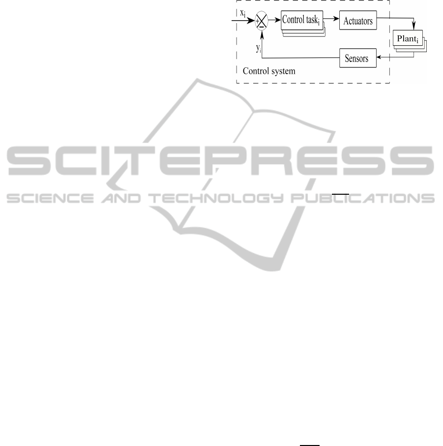
A typical embedded real-time control system is com-

posed (as illustrated in Figure 1) of plants to be con-

trolled, actuators, sensors and a set of N control tasks

Γ = {τ

| 1 ≤ i ≤ N} which are independent and

fully preemptible. Each task is responsible for con-

trolling an independent physical process (plant). The

tasks run concurrently over the same shared proces-

sor.

Figure 1: Embedded real-time control system.

Assume that the processor has M

discrete operating frequencies f

{ f

|1 ≤ m ≤ M, f

min

= f

< ... < f

= f

max

We deﬁne a scaling factor or processor speed S

the normalized frequency of f

with respect to the

maximum frequency f

max

, that is :

max

(1)

We use EDF scheduling policy (Liu and Layland,

1973) where the task priority is proportional to its ur-

gency. A task τ

is characterized by the following in-

dependent parameters :

• r

, the ﬁrst release time of the task τ

; a task in-

stance is named a job τ

i,k

, k > 0. The job τ

i,0

released at the date r

i,0

= r

= 0;

• T

the release period of the task τ

: ev-

ery subsequent job τ

i,k

is released at the date

i,k

= (k − 1) × T

, k > 0. By default, we

consider the relative deadline of a control task to

be equal to its period;

• e

, the absolute error of the task τ

: is deﬁned

as the absolute difference between the reference

input x

and the plant output y

, i.e., e

=| x

− y

In order to compare the solution givenin this work

to other ones based on tasks parameters, we deﬁne the

following additional parameter :

• U

inst

(t) =

∑

i=1

i,1

(t)

, as the instantaneous proces-

sor utilization. The term C

i,1

(t) is equal to the lat-

est estimated execution time of task τ

at time t ac-

cording to the low-passﬁlter proposed by (Cervin,

2003).

4.2 Energy Consumption Model

We are concerned with the DVFS technique which

is able to reduce the dynamic power dissipation of a

CMOS integrated circuit, such as a modern computer

AReal-TimeFeedbackSchedulerbasedonControlErrorfor

EnvironmentalEnergyHarvestingSystems

351

processor, by reducing the frequency at which it op-

erates. The dynamic power dissipation is given by :

P = C × v

× f, where C denotes the effective switch

capacitance related to the type of processor, f is the

frequency and v is the voltage.

In this work, we based our study on the commer-

cial processor XScale (XScale, 2007). Its main char-

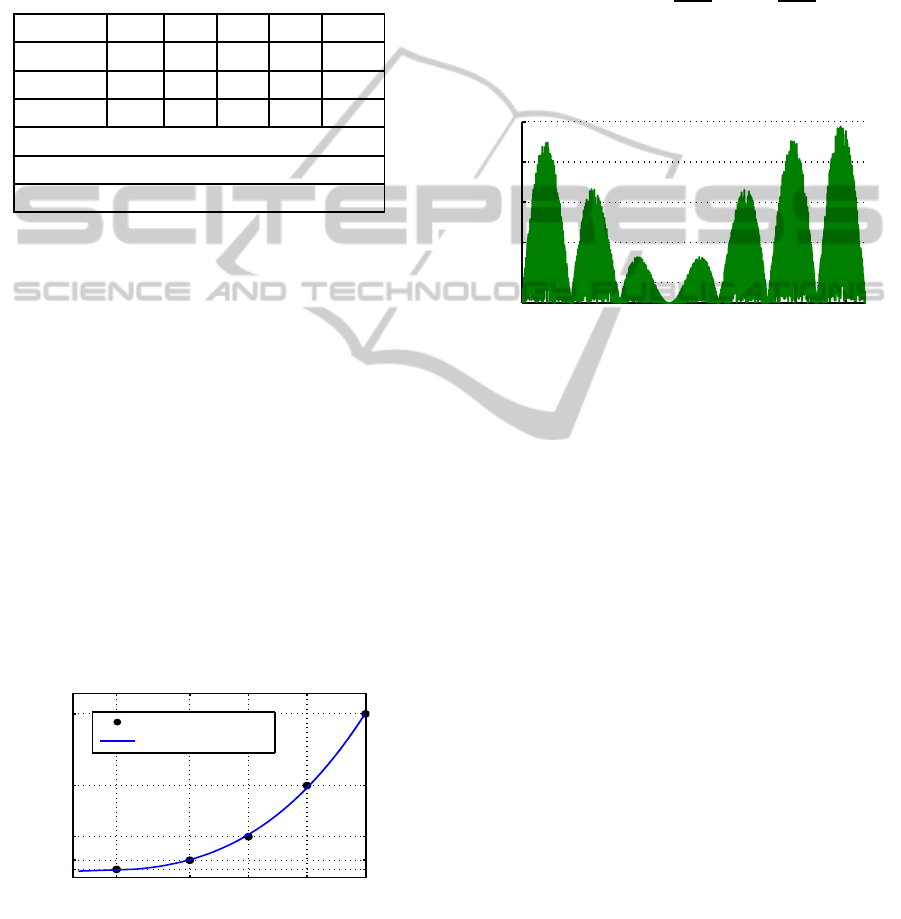
acteristics are given in Table 1 (Xu et al., 2007).

Table 1: XScale Parameters.

V(V) 0.75 1.0 1.3 1.6 1.8

F(MHz) 150 400 600 800 1000

0.15 0.4 0.6 0.8 1

P(mW) 80 170 400 900 1600

Energy switch (1.2 µJ)

Switch time (12 µs)

Idle Power (mW) (63.85 )

We want to compare an algorithm that assumes

continuous change with others assume discrete fre-

quency changes so we need a model of continuous

consumption. According to the relation derived in

(Xu et al., 2007), several power models of this proces-

sor are cited in the literature. Those models describe

the power consumption as a polynomial function of

the processor speed S. We selected the model pre-

sented in (Chen et al., 2013) where the active power

function is written as :

P = 1543.28× S

2.87

+ 63.85 (2)

Figure 2 shows that the continuous approximation

of the power consumed depending on the frequency,

is ﬁtting with the constructor discrete power over fre-

quency values. Therefore, the function shown in Fig-

ure 2 appears to be as realistic as possible, if we were

to assume the existence of a XScale processor able to

change its frequency continuously.

0.15 0.4 0.6 0.8 1

170

400

900

1600

Normalized Frequency

Power [mW]

Actual power

63.58+1543.28*S

2.87

Figure 2: Power Consumption function.

For a time interval [t

], the energy consumption

is given by Ec(t

) =

P(S(t))dt.

4.3 Energy Source Model

We assume that the environmental energy, such as so-

lar energy, is harvested and converted into electrical

energy to supplement the battery of an embedded sys-

tem. The solar energy source behavior is modelized

as follows (Moser et al., 2007) :

Ps(t) = |0.9R(t) × cos(

0.7π

) × cos(

0.1π

)| (3)

where R(t) denotes a uniform distributed random

variable between 0 and 1. The values of Ps have been

cutted off at the value Ps,max = 0.9.

1 2 3 4 5 6 7

0.1

0.3

0.5

0.7

0.9

Time

Ps(t)

Figure 3: Power trace Ps(t).

As shown in Figure 3, the obtained power trace

Ps(t) is simulating periods similar to those experi-

enced by solar cells in an outdoor environment.

The input power Ps(t) has excluded the loss in-

curred by auxiliary circuitry. In other words, Ps(t) is

the net power to feed the storage unit. The total en-

ergy, Es(t

), that is harvested in the time interval

] is given by Es(t

) =

Ps(t)dt.

The system uses an energy storage unit with nom-

inal capacity, (E, expressed in Joules or Watts-hour).

The energy level, denoted as El(t) at a given time t,

has to remain between two boundaries E

min

and E

max

If the storage is fully discharged, no task can be ex-

ecuted, and the processor has to be stopped. In con-

trast, if the storage is fully charged, and we continue

to charge it, energy is wasted. To reduce waste and

to ensure QoC, it would be useful to perform tasks at

the maximum CPU speed when the battery is ”almost

full”.

5 FEEDBACK SCHEDULING

BASED ON CONTROL ERROR

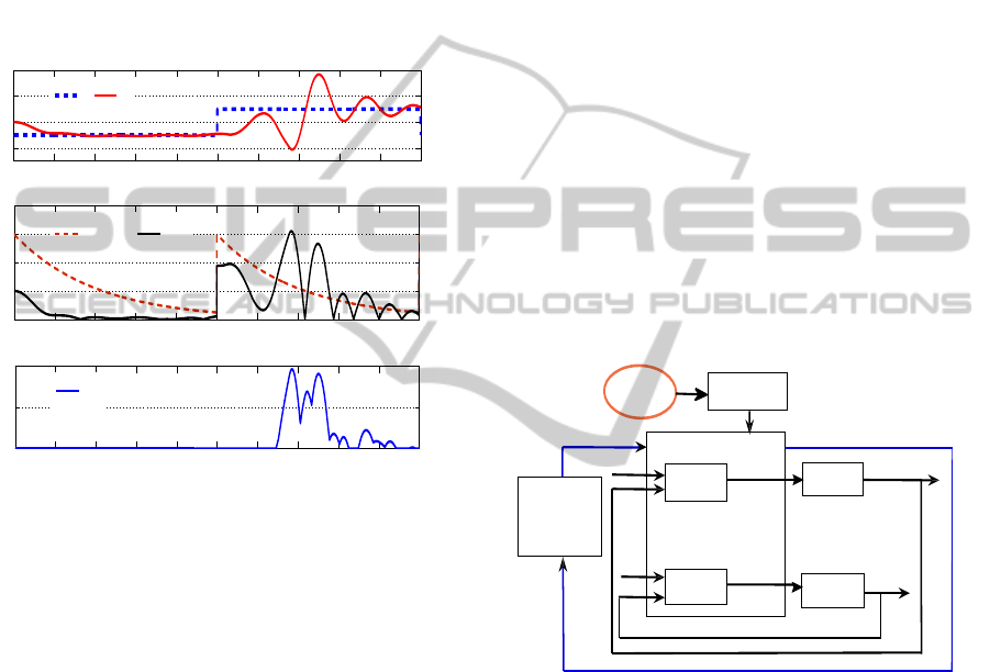
5.1 Control Cost Model

Assume that the reference signal x

is a square signal

whose period is 2h. The reference signal is run during

PECCS2015-5thInternationalConferenceonPervasiveandEmbeddedComputingandCommunicationSystems

352

periods. From a control standpoint, the error be-

tween the reference signal x

and the measured signal

should mirror how good is the control strategy (see

Figure 4 (a)). If we include a decay constraint on the

error we impose by the same way a relative degree of

stability. It is more appropriate to impose (see Figure

4 (b)), at each half signal period, an exponential decay

on the error by forcing the absolute value of the error

to lie inside an envelope limited by a function of the

form: f(t) = k

− α t

, where the parameters k

and

α have to be chosen appropriately by the designer. k

and α deﬁne the desired relative stability degree.

0 0.1 0.2 0.3 0.4 0.5 0.6 0.7 0.8 0.9 1

−2

(a)

0 0.1 0.2 0.3 0.4 0.5 0.6 0.7 0.8 0.9 1

(b)

f(t)=k

− α t

i, k

(t)

0 0.1 0.2 0.3 0.4 0.5 0.6 0.7 0.8 0.9 1

(c)

(t)

Figure 4: Parameters illustration of the control cost model.

To appropriately measure the QoC at the execution of

the job τ

i,k

at time t, we deﬁne the control cost as :

i,k

(t) =sup



0 ; e

(t) − k

−α(t−(q−1)h)



with 1 ≤ q ≤ 2N

(4)

where h is the duration of the half period of the refer-

ence signal, N

is the running periods, k

−α(t−(q−1)h)

is the exponential decay function imposed at the q

half period of the reference signal, e

(t) is the abso-

lute error of the task τ

at time t. The idea is to con-

sider at each execution of the job τ

i,k

only the positive

value of the difference between the absolute error and

exponential decay function (see Figure 4 (b)).

We assume the FBS task to be executed periodi-

cally with a period T

. We deﬁne the control cost of

the control task τ

at the j

(j > 0) execution of the

FBS task as :

( j−1)T

i,k

(t)dt (5)

The idea is to compute the control cost of the control

task τ

between two consecutive executions of FBS

task. Note that I

allows to measure how far is the i

plant from an acceptable behavior. It provides enough

information about plant stability (see Figure 4 (c)).

We assume that if the value I

is not null, the corre-

sponding plant is unstable.

For N control tasks, we deﬁne the maximum con-

trol cost of the control system as :

sys

Max

1≤i≤N

(6)

The use of the Max function is motivated by the

will to give greater attention to the unstable plant.

5.2 Feedback Scheduling Framework

The framework of the proposed scheme is shown in

Figure 5. Aside from the control loops, an outer

feedback loop is introduced to implement feedback

scheduling. The basic role of the feedback scheduler

is to use the amount of available energy and the con-

trol cost given by Eq.6 of each control task as the

feedback information in order to compute a discrete

frequency for the processor.

Plant N

Plant 1

CPU

Feedback

scheduling

Energy

Source

B a tte ry

Task 1

Scaling factor

Control cost

Energy available

and

Task N

Figure 5: Scheme of the feedback scheduler.

5.3 Presentation of the Algorithm

The objective of our work is to propose a heuristic

(see Algorithm 1) called FSCE-EH (Feedback Sched-

uler based on Control Error for Energy Harvesting)

enabling the execution of tasks with a speed just

above current speed if maximum control cost of the

system I

sys

(see Eq. 6) is greater than 0. Otherwise,

the FSCE-EH returns current speed as a new speed

if the amount of available energy is greater than

a threshold set off-line. The FSCE-EH algorithm

returns a speed just below current speed when I

sys

is null and the available energy level is below this

threshold.

AReal-TimeFeedbackSchedulerbasedonControlErrorfor

EnvironmentalEnergyHarvestingSystems

353

Assuming El(t) the amount of available energy in

the battery at time t, I

sys

the maximum control cost of

the system (see Eq. 6), L the energy threshold and

the current speed (scaling factor) S(k). The new speed

S is given by the algorithm below :

Algorithm 1: FSEC-EH.

Input:

El(t), the amount of energy available;

sys

, the maximum control cost of the system

(see Eq.6);

L, the threshold ;

S(k), the current speed (see Eq.1);

Output:

S, the scaling factor required

1 if I

sys

> 0 then

2 S ← S(k+ 1)

3 else

4 if El(t) > L then

5 S ← S(k)

6 else

7 S ← S(k− 1)

8 return S;

6 PERFORMANCE RESULTS

This section presents the simulation experiments us-

ing TrueTime (Cervin et al., 2010). Simulations aim

to evaluate the QoC of the proposed scheme.

6.1 Environment and Simulation

Context

For our experiments, a power generator source which

supplies a battery according to the model given in

Eq.(3) is implemented in TrueTime (Cervin et al.,

2010). We consider an embedded control system that

consists of three independent control loops. Each

plant is controlled using a PID algorithm whose

parameters are similar to those given in (Cervin

et al., 2010). The transfer function of each plant is

G(s) = 1000/(s

+ s). For this, we consider the set

of three tasks Γ = {τ

| 1 ≤ i ≤ 3}. In our experiments,

the nominal sampling periods of three loops are set to

be T

= 15 ms, T

= 16 ms, and T

= 17 ms, respec-

tively. The power consumption of the task τ

under

the processor speed S is given in Eq. (2), with the

processor idle power equal to 63.58 mW. We assume

that the energy storage capacity is E

max

= 2.5 Joules

at t = 0. The FBS task period is equal to T

= 80 ms.

We assume that at t = 0 the processor speed is S = 1.

In our simulation, the reference signal was run dur-

ing Nr = 55 periods. The parameters of the stability

degree are k

= 3 and α = 5

Based on the above description, we compare the

proposedfeedback scheduling method (FSCE-EH) to

the three following methods :

1. EDFnoDVFS: The processor operates at its full

speed (S = 1) under the classical EDF policy,

i.e., there is no DVFS scheme and no feedback

scheduling;

2. EDFbs-EgC: Earliest Deadline Feedback

Scheduling with Energy guarantee under Con-

tinuous voltage/frequency modes algorithm,

proposed in (Abbas et al., 2013) in which the

scaling factor S takes a value S = U

inst

(t) at each

execution of the FBS task;

3. FS-EH (Feedback Scheduler with Energy Har-

vesting): heuristic proposed in (Abbas et al.,

2014) in which the scaling factor S takes

a value S = 1 at each execution of the

FBS task if the amount of available energy is

greater than a threshold (set ofﬂine), otherwise

S = min{ S

| S

≥ max(U

inst

(t),El(t)/L)}.

6.2 Results and Discussions

In this section we present results of the simulations for

the four methods previously listed. Each simulation

has been performed during 55 s. With the aim to show

the effect of the choice of the threshold, we chose 25

different values for the threshold L from 0.1 to 2.5

(battery nominal capacity).

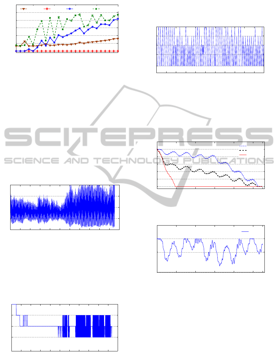
6.2.1 Average and Minimum Energy Available

We show here, for each threshold value, the average

and minimum energy available during the experiment.

When FSCE-EH and FS-EH are used, Figure 6

shows that the increases of the average energy avail-

able with the increase of threshold values. Accord-

ing to experiments, we found that when the thresh-

old value is spread over the entire battery capacity

(equal to 2.5) provides a high average energy avail-

able. We can see also that the minimum energy avail-

able is equal to 0 with FS-EH for all threshold values

caused by the total discharge of the battery which in-

duces the experiment stop. We note that the average

energy available with EDFnoDVFS and EDFbs-EgC

are equal to 0.36 J and 1.53 J, respectively. The min-

imum energy available with the two last algorithms is

equal to 0.

PECCS2015-5thInternationalConferenceonPervasiveandEmbeddedComputingandCommunicationSystems

354

0,1 0,5 1 1,5 2 2,5

0,5

1,5

2,5

Average and Minimum

Energy available

Threshold values

Aver FS−EH Min FS−EH Min FSCE−EH Aver FSCE−EH

Figure 6: Average and Minimum Energy available vs

Threshold with FSCE-EH and FS-EH.

6.2.2 Processor Speed Comparison

In this section, we present results showing the proces-

sor frequency variation with each method presented

previously. We note that there is an overhead in time

and energy for every frequency change (see Table.

2). We note also that when FSCE-EH and FS-EH are

used, the threshold take value equal to 2.5

From Figure 7, we can see that under EDFbs-

EgC algorithm the processor frequency is changing

rapidly. The frequent change in processor frequency

from low values to high values induces less reduction

in energy consumption (see Figure 10).

0 5 10 15 20 25 30 35 40 45 50 55

0.2

0.4

0.6

0.8

Times [s]

Scaling Factor

Figure 7: Scaling Factor with EDfbs-EgC.

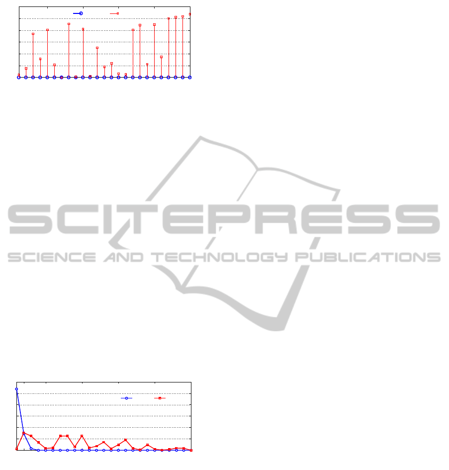
Figure 8 shows that when FS-EH algorithm is

used, a frequent change in processor frequency occur.

We note that with EDFbs-EgC (resp. with FS-EH)

algorithm the execution stop due to the battery dis-

charge at t = 52.7 s (resp. t = 54.4 s) which causes

the destabilization of controlled plant.

0 5 10 15 20 25 30 35 40 45 50 55

0.15

0.4

0.6

0.8

Times [s]

Scaling Factor

Figure 8: Scaling Factor with FS-EH.

Figure 9 shows that when FSCE-EH algorithm is

used, the execution does not stop. We can see also

that FSCE-EH algorithm returns a lower speed (0.15)

to favor the charge of the battery and return also a the

high speed (1) to improve control performance.

0 5 10 15 20 25 30 35 40 45 50 55

0.15

0.4

0.6

0.8

Times [s]

Scaling Factor

Figure 9: Scaling Factor with FSCE-EH.

6.2.3 Energy Consumption Comparison

Figures 10 and 11 show the energy available with the

four methods. We can see that FSCE-EH protects

against a total discharge of the battery.

0 10 20 30 40 50 55

0.5

1.5

2.5

Times [s]

Energy available

EDFbs−EgC

FS−EH

EDFnoDVFS

Figure 10: Energy available with EDFnoDVFS, EDfbs-EgC

and FS-EH.

0 10 20 30 40 50 55

2,3

2,5

Times [s]

Energy available

FSCE−EH

Figure 11: Energy available with FSCE-EH.

6.2.4 Rate of Missed Deadlines Comparison

We present results concerning the rate of missed dead-

lines that is the number of deadlines missing divided

by the total number of jobs.

Figure 12 shows that under FSCE-EH a small rate

of deadlines are missed. The maximum (resp. mean)

rate of missed deadlines is 10.74% (resp. 4.96%)

comparatively to the rate under FS-EH which equals

to 0. With EDFbs-EgC algorithm the rate of missed

deadlines is 0.37%.

AReal-TimeFeedbackSchedulerbasedonControlErrorfor

EnvironmentalEnergyHarvestingSystems

355

0,1 0,5 1 1,5 2 2,5

Rate of missed deadlines(%)

Threshold values

with FS−EH with FSCE−EH

Figure 12: Rate of missed deadlines under FSCE-EH and

FS-EH.

6.2.5 Quality of Control Comparison

The Integral of Absolute Error (IAE) for each closed

loop system i, i.e J(i) =

sim

(t)dt measures the

QoC (Quality of Control), where e

is the absolute

control error. For an experiment, we deﬁne the maxi-

mum error cost as : J

Max

1≤i≤3

J(i).

Figure 13 shows the maximum error cost J

Max

with FSCE-EH and FS-EH for each threshold value.

We can see that FSCE-EH algorithm induce less cost

comparatively to the cost induced bay FS-EH algo-

rithm. We note that the minimum J

Max

under FS-

EH is equal to 375330 obtained with threshold value

equal to 2.5. Under FSCE-EH, the minimum J

Max

equal to 63393 (which is 16.9% less) obtained with

threshold value equal to 0.7. We note also that under

EDfbs-EgC the maximum error cost J

Max

is equal to

906100. These results show that the FSCE-EH algo-

rithm optimizes the QoC even if it induces small rate

of missed deadlines (see Figure 12).

0,1 0,2 0,5 1 1,5 2 2,5

x 10

Error cost

Threshold values

FSCE−EH FS−EH

Figure 13: Maximum error cost J

Max

with FSCE-EH and

FS-EH.

7 CONCLUSIONS

This paper has addressed the problem of real-time

scheduling in ambient energy harvesting systems with

discrete voltage/frequency modes through the use of a

feedback scheduler. The proposed solution computes

the processor speed with taking into accountthe avail-

able energy and the control performance. The eval-

uation of this solution shows experimentally a good

compromise between the available energy and the

quality of control and we can say that our approach

is promising.

In the near future, we plan to study the problem of

scheduling hybrid tasks (hard and soft real-time task)

under harvesting energy constraints. The objective is

to guarantee, with energy saving, the hard real-time

constraints and at the same time reduce the rate of

missed deadlines for the soft real-time tasks. We plan

also to improve and test our work on a real hardware.

REFERENCES

Abbas, A., Grolleau, E., Loudini, M., and Mehdi, D. (2013).

A real-time feedback scheduler for environmental en-

ergy harvesting. In Systems and Control (ICSC), 2013

3rd International Conference on, pages 1013–1019.

Abbas, A., Grolleau, E., Mehdi, D., Loudini, M., and Hi-

douci, W.-K. (2014). A real-time feedback sched-

uler for environmental energy with discrete volt-

age/frequency modes. In The 2nd International Con-

ference on Future Internet of Things and Cloud. IEEE.

Arz´en, K.-E., Robertsson, A., Henriksson, D., Johansson,

M., Hjalmarsson, H., and Johansson, K. H. (2006).

Conclusions of the artist2 roadmap on control of com-

puting systems. SIGBED Review, 3(3):11–20.

Axer, P., Ernst, R., Falk, H., Girault, A., Grund, D., Guan,

N., Jonsson, B., Marwedel, P., Reineke, J., Rochange,

C., Sebastian, M., Hanxleden, R. V., Wilhelm, R., and

Yi, W. (2014). Building timing predictable embedded

systems. ACM Transactions on Embedded Computing

Systems, 13(4).

Cervin, A. (2003). Integrated Control and Real-Time

Scheduling. Phd thesis, Lund University.

Cervin, A., Henriksson, D., and Ohlin, M. (2010). True-

time: Reference manual.

Chen, G., Huang, K., Huang, J., Buckl, C., and Knoll,

A. (2013). Effective online power management with

adaptive interplay of dvs and dpm for embedded real-

time system. In DSD, pages 881–889.

Chetto, M. (2014). Optimal scheduling for real-time jobs

in energy harvesting computing systems. IEEE Trans-

actions on Emerging Topics in Computing, 2(2):122–

133.

Chetto, M. and Zhang, H. (2010). Performance evaluation

of real-time scheduling heuristics for energy harvest-

ing systems. In Green Computing and Communica-

tions (GreenCom), 2010 IEEE/ACM Int’l Conference

on Int’l Conference on Cyber, Physical and Social

Computing (CPSCom), pages 398–403. IEEE Com-

puter Society.

Jin, H., Wang, D., Wang, H., and Wang, H. (2007). Feed-

back fuzzy-dvs scheduling of control tasks. The Jour-

nal of Supercomputing, 41(2):147–162.

Liu, C. L. and Layland, J. W. (1973). Scheduling algo-

rithms for multiprogramming in a hard-real-time en-

vironment. Journal of the ACM (JACM), 20(1):46–61.

PECCS2015-5thInternationalConferenceonPervasiveandEmbeddedComputingandCommunicationSystems

356

Liu, S., Lu, J., Wu, Q., and Qiu, Q. (2012). Harvesting-

aware power management for real-time systems with

renewable energy. IEEE Transactions on Very Large

Scale Integration (VLSI) Systems, 20(8):1473–1486.

Liu, S., Qiu, Q., and Wu, Q. (2008). Energy aware dynamic

voltage and frequency selection for real-time systems

with energy harvesting. In Proceedings of the Con-

ference on Design, Automation and Test in Europe,

DATE ’08, pages 236–241.

Liu, S., Wu, Q., and Qiu, Q. (2009). An adaptive schedul-

ing and voltage/frequency selection algorithm for real-

time energy harvesting systems. In Design Automa-

tion Conference, 2009. DAC’09. 46th ACM/IEEE,

pages 782–787. IEEE.

Moser, C., Brunelli, D., Thiele, L., and Benini, L. (2007).

Real-time scheduling for energy harvesting sensor

nodes. Real-Time Systems, 37(3):233–260.

Soria-Lopez, A., Mej´ıa-Alvarez, P., and Cornejo, J. (2005).

Feedback scheduling of power-aware soft real-time

tasks. In ENC, pages 266–273.

Xia, F. (2006). Feedback scheduling of real-time control

systems with resource constraints. Phd thesis, Zhe-

jiang University.

Xia, F., Ma, L., Zhao, W., Sun, Y., and Dong, J. (2008). En-

hanced energy-aware feedback scheduling of embed-

ded control systems. arXiv preprint arXiv:0809.4917.

XScale (2007). Intel xscale microarchitecture.

Xu, R., Moss´e, D., and Melhem, R. (2007). Minimiz-

ing expected energy consumption in real-time systems

through dynamic voltage scaling. ACM Trans. Com-

put. Syst., 25(4).

AReal-TimeFeedbackSchedulerbasedonControlErrorfor

EnvironmentalEnergyHarvestingSystems

357