Combination of Characteristic Green’s Function Technique and Rational

Function Fitting Method for Computation of Modal Reﬂectivity

at the Optical Waveguide End-facet

Abdorreza Torabi and Amir Ahmad Shishegar

Department of Electrical Engineering, Sharif University of Technology, Tehran, Iran

Keywords:

Optical Waveguide End-facet, Guided Mode Reﬂection Coefﬁcient, Characteristic Green’s Function, Complex

Images Method, Rational Function Fitting Method, VECTFIT Algorithm, Optimization.

Abstract:

A novel method for computation of modal reﬂectivity at optical waveguide end-facet is presented. The method

is based on the characteristic Green’s function (CGF) technique. Using separability assumption of the struc-

ture and rational function ﬁtting method (RFFM), a closed-form ﬁeld expression is derived for optical planar

waveguide. The uniform derived expression consists of discrete and continuous spectrum contributions which

denotes guided and radiation modes effects respectively. An optimization problem is then deﬁned to calculate

the exact reﬂection coefﬁcients at the end-facet for all extracted poles obtained from rational function ﬁtting

step. The proposed CGF-RFFM-optimization offers superior exactness in comparison with the previous re-

ported CGF-complex images (CI) technique due to contribution of all components of ﬁeld in the optimization

problem. The main advantage of the proposed method lies in its simple implementation as well as precision

for any refractive index contrast. Excellent numerical agreements with rigorous methods are shown in several

examples.

1 INTRODUCTION

Optoelectric devices such as laser ampliﬁer, opti-

cal modulator and coupler are widely used in in-

tegrated optics (IO) circuits. In these applications,

facet reﬂectivity typically deviates the performance of

the integrated system from its original designed tar-

get. The oldest accepted model for computation of

facet reﬂectivity is Ikegami’s model (Ikegami, 1972),

which was introduced for double-heterojunction(DH)

GaAs-AlGaAs lasers. In this approach, with the use

of eigenmode expansion, electric and magnetic ﬁelds

are matched at the facet. In (Lewin, 1975), an ap-

proximate modal reﬂectivityis developedby means of

a plane wave Fresnel reﬂectivity expansion. Derived

expressions are utilized in some other works related

to two-dimensional (2-D) buried DH lasers (Hardy,

1984). These results are quite accurate but are just

useful for low refractive index contrast. Gelin (Gelin

et al., 1981) extended Rozzi’s variational treatment

(Rozzi and Veld, 1980) for end-facet modal reﬂec-

tivity and proposed an efﬁcient numerical computa-

tion. The main challenge of mode matching based

approach is the computation of time-consuming inte-

grals which usually have singular integrands to con-

tribute radiation modes. Moreover, ﬁnite window

Fourier transform could be combined with perturba-

tion series for fast computation of end-facet reﬂectiv-

ity (Chen et al., 2012).

An efﬁcient way to regard the continuous spec-

trum contribution in mode matching method is using

appropriate set of modes achieved by closing the de-

sired structures with perfectly matched layers (PMLs)

(Derudder et al., 2001). The main disadvantage of

PML method is the considerable number of discrete

modes must be considered to obtain for an appropri-

ate accuracy. A different approach is utilizing itera-

tive based methods. In (Yevick et al., 1991), split-

operator method is utilized and the interface of facet is

divided into segments in such a way that within each

segment the refractive index is nearly constant. The

resulting contribution of each segment to the total re-

ﬂected ﬁeld is superimposed. Finally a linear iterative

equation is obtained which can be solved by classi-

cal Neumann series or more stably by bi-conjugate

gradient method (Wei and Lu, 2002). In other it-

erative approach, reﬂection operator is diagonalized

completely or partially (Yevick et al., 1992) using the

known eigenmodes and eigenvectors of square root

operator. A separate class of solution methods em-

Torabi A. and Shishegar A..

Combination of Characteristic Green’s Function Technique and Rational Function Fitting Method for Computation of Modal Reﬂectivity at the Optical

Waveguide End-facet.

DOI: 10.5220/0005332300140021

In Proceedings of the 3rd International Conference on Photonics, Optics and Laser Technology (PHOTOPTICS-2015), pages 14-21

ISBN: 978-989-758-093-2

 2015 SCITEPRESS (Science and Technology Publications, Lda.)

ploy Pad´e or complex Pad´e approximations to ratio-

nal approximation of the square root operator (El-

Refaei et al., 2000), (Jamid and Khan, 2007), (Yu and

Yevick, 1997). Stability and convergenceproblem are

the main challenges in this approach. For more rig-

orous solution, integral equation can be used. Parsa

and Paknys (Parsa and Paknys, 2007a) used equiva-

lence principle and image theory and model the trun-

cated semi-inﬁnite dielectric slab waveguide by an

inﬁnite dielectric slab with unknown current density

on a plane just at truncating surface of the end-facet

which is solved by the method of moments (MoM).

Coupling of the guided modes are incorporated in this

method in the form of coupling matrix of end-facet.

In this paper a novel method for computation of

guided modes reﬂectivity at the waveguide end-facet

is presented. The proposed method is based on the

characteristic Green’s function (CGF) technique com-

bined with rational function ﬁtting method (RFFM)

(Torabi et al., 2014b), (Torabi et al., 2013). Spa-

tial Green’s function of ﬁnite dielectric planar waveg-

uide is obtained by separation of the structure into

inﬁnite 1-D layered media. For nonseparable struc-

ture like typical ﬁnite dielectric slab waveguide (i.e.

DH laser), using separability assumption, an approx-

imate and closed-form expression for spatial Green’s

function is achieved. The ﬁnal formulation is utilized

in an efﬁcient optimization problem to ﬁnd the ex-

act facet reﬂection coefﬁcients of guided modes. In

contrary to previous reported CGF-complex images

( , )

x y

′ ′

−

(a)

( , )

x y

′ ′

(b)

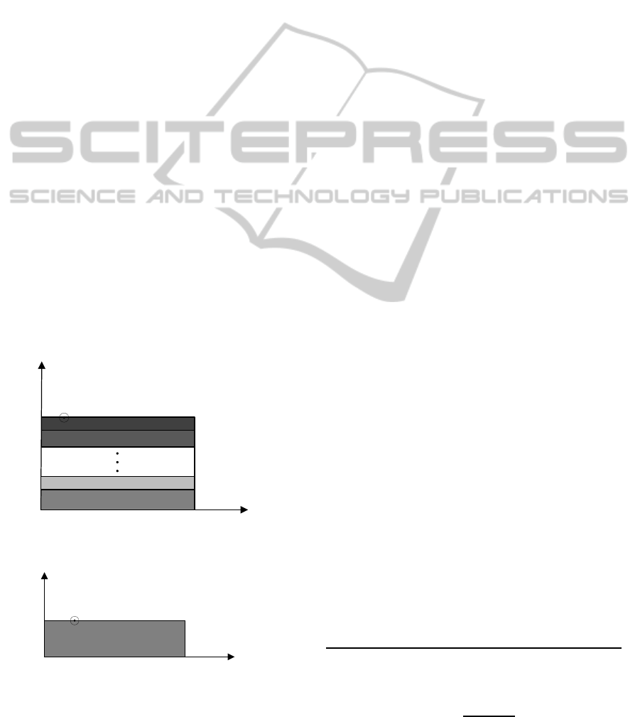
Figure 1: A line source on a truncated (a) multilayered (b)

slab waveguide.

(CI) based method (Torabi et al., 2014a), in the for-

mulation of CGF-RFFM continuous spectrum contri-

bution are presented by some poles similar to guided

modes part. Then unlike CGF-CI, in CGF-RFFM

both discrete and continuous spectrum contributions

are efﬁciently incorporated in the optimization prob-

lem. Therefore more exact results of guided modes

reﬂectivity can be obtained. This fact is shown in sev-

eral examples. Simplicity of implementation as well

as precision is the main advantage of the proposed

method. Moreover, this method can be used for any

planar dielectric waveguides with abrupt termination

and also for any refractive index contrasts.

2 CGF-RFFM FORMULATION

2.1 CGF Technique and Separability

Assumption

The 2-D Helmholtz’s equation should be solved for

Green’s function of magnetic vector potential, A

, for

a line source surrounded by layered media as it is

shown in Fig. 1(a). Here for simplicity the derivations

are developed for truncated dielectric slab waveguide

shown in Fig. 1(b) for simplicity while the implemen-

tation for multilayered media (Fig. 1(a)) is straight-

forward. The 2-D Helmholtz’s equation can be sepa-

rated into two 1-D equations if (Faraji-Dana, 1993a),

(Shishegar and Faraji-Dana, 2003)

(x,y) = ε

(x) + ε

(y). (1)

By the assumption of (1), the original structure has

been decomposed into two layered media denoted by

and N

layered media (Fig. 2(a) and Fig. 2(b), N

called normal to γ where γ = x,y), which their relative

dielectric constants are ε

(x) and ε

(y) respectively.

If this separation is rigorously possible, it means that

the original structure, Fig. 1(b), can be exactly repro-

duced by crossing two 1-D N

and N

layered me-

dia which is shown in Fig. 2(c). The solutions to

the 1-D Helmholtz’s equations are denoted by G

(for

Fig. 2(a)) and G

(for Fig. 2(b)) and can be obtained

analytically using usual spectral techniques (Michal-

ski and Mosig, 1997). We will have,

(γ,γ

′

) =

(1+ R

−j2β

γ1

)(1+ R

−j2β

γ1

−γ

)

−jβ

γ1

(γ

−γ

)

(2jβ

γ1

)(1−R

−j2β

γ1

)

(2)

γ1

−β

γ2

γ1

+ β

γ2

, (3)

CombinationofCharacteristicGreen'sFunctionTechniqueandRationalFunctionFittingMethodforComputationof

ModalReflectivityattheOpticalWaveguideEnd-facet

where d

is equal to w and t for γ = x and y respec-

tively. γ

and γ

are greater and smaller values of γ

and γ

′

respectively and β

γi

+ λ

(i = 1,2).

and R

are the reﬂection coefﬁcients of a TE wave

at the interfaces (due to the symmetry R

= R

and R

= R

in Fig. 2). Then having G

and G

, the solution of A

for separable structure of

Fig. 2(c) is given by (Faraji-Dana, 1993a), (Shishegar

and Faraji-Dana, 2003)

(x,y;x

′

)

= (

−1

2π j

)

(x,x

′

,−λ

(y, y

′

,λ

)dλ

(4)

where the contourC

, encloses only the singularities

of G

, (including branch cut, branch point and dis-

crete poles singularities), in counterclockwise sense.

For the structure at hand, Fig. 1(b), it can be shown

that the separation of (1), is not rigorously possi-

ble (Shishegar and Faraji-Dana, 2003). If one ig-

nore (1) in four exterior regions in Fig. 2(c), then

an inﬁnite number of solutions for ε

, ε

and

could be found. It must be noted that the so-

lutions are not physically available relative dielec-

tric constants. They are just mathematical quantities.

One can choose ε

= 0, ε

= ε

−ε

, ε

= ε

for N

and N

media. For all possible so-

lutions, the corner regions of the original structure

are replaced by ε

+ ε

= 2ε

−ε

(Shishegar and

Faraji-Dana, 2003). This deviation makes the CGF

result in (4) an approximate Green’s function for orig-

inal structure (Fig. 1(b)). It should be noted that for

multilayered truncated waveguide (with n layers) of

Fig. 1(a), after separation, the N

layered media would

be a 1-D inﬁnite layered media (with n layers) while

media would be the same as Fig. 2(a). So it is just

sufﬁcient that G

of related N

layered media is com-

puted analytically and incorporated in integral repre-

sentation of (4).

2.2 CGF-RFFM

In common optical waveguide structures, t is much

smaller than w. So, with acceptable approxima-

tion, guided modes (surface wave poles) of CGF G

(Fig. 2(b)) denote the guided modes of the original

structure in Fig. 1(b). Furthermore, the integration

of (4) in CGF technique is so time consuming and

expensive due to highly oscillatory nature of its in-

tegrand. To circumvent the numerical integration of

(4), rational function ﬁtting method can be used. In

CGF-RFFM the G

is ﬁrst approximated by appropri-

ate set of discrete poles via modiﬁed VECTFIT algo-

A x

(a)

A y

(b)

1 1

x y

ε ε

( , )

x y

′ ′

1 2

x y

ε ε

1 2

x y

ε ε

2 1

x y

ε ε

2 2

x y

ε ε

2 2

x y

ε ε

2 1

x y

ε ε

2 2

x y

ε ε

2 2

x y

ε ε

(c)

Figure 2: (a) N

and (b) N

layered media, (c) Separable

structure analyzed instead of original structure in CGF tech-

nique.

rithm (Torabi et al., 2014b). Like,

(y, y

′

,λ

) ≈

∑

m=1

Res

−λ

(5)

where Res

is the residue of G

at the mth pole. N

is the number of poles used in RFFM for rational ﬁt-

ting. It should be noted that the set of extracted poles

in (5) includes guided modes of the structure. More-

over, some other poles are also extracted that are re-

sponsible to construct the continuous spectrum con-

tribution. Therefore, these poles have similar char-

acteristic to leaky wave poles and so we may call

them quasi leaky wave poles (Torabi et al., 2014b).

Then by substituting (5) in (4) and applying residue

theorem, a closed form series representation for A

will be obtained and can be found by (6). In (6),

−λ

is the propagation constant of

the mth mode in the x-direction. Since the rational

function ﬁtting of (5) would have excellent accuracy,

therefore a closed form relation of (6) can approx-

imate the integral of (4) very well. We can sepa-

rate A

of (6) in two terms like (7) where A

denotes

the guided modes part (or discrete spectrum contribu-

tion) and is in series form of (6) in which just guided

modes (surface wave poles) contributes while A

re-

lated to radiation modes part (or continuous spectrum

contribution) and is in series form of (6) in which the

non surface wave poles (quasi leaky wave poles) con-

tributes.

In (6), R

is the reﬂection coefﬁcient of modes

PHOTOPTICS2015-InternationalConferenceonPhotonics,OpticsandLaserTechnology

∑

m=1

−Res

(1+ R

−j2k

)(1+ R

−j2k

(w−x

)

−jk

−x

)

(2jk

)(1−R

−j2k

)

, (6)

= A

+ A

guided

∑

m=1

−Res

(1+ R

−j2k

)(1+ R

−j2k

(w−x

)

−jk

−x

)

(2jk

)(1−R

−j2k

)

−N

guided

∑

m=1

−Res

(1+ R

−j2k

)(1+ R

−j2k

(w−x

)

−jk

−x

)

(2jk

)(1−R

−j2k

)

(7)

at the N

interface shown in Fig. 3(a). But actually,

these modes are reﬂected from truncated surface of

the substrate shown in Fig. 3(b). This discrepancy

arises from the separability approximation of the orig-

inal structure which also makes the refractive index of

four exterior corners deviate from its exact value. For

low refractive index contrast, ε

≈ ε

, as is common

in optical buried waveguides, the error in A

due to ap-

proximate modeling of the corner regions is ignorable

because 2ε

−ε

≈ ε

. But in high refractive index

contrasts, considerable deviation may be imposed on

the Green’s function especially for source and ﬁeld

points close to the corners. Therefore to have exact

for truncated dielectric slab waveguide of Fig. 1(b)

both terms A

and A

should be corrected. Although

having enough distance from corners for source and

ﬁeld point makes the deviation in A

part small but

for more accurate results of reﬂection coefﬁcients of

guided modes, correction of A

part along with A

part

should be considered. Before deﬁning the optimiza-

tion problem, it should be noted that the main dif-

ference between proposed CGF-RFFM and CGF-CI

method (Torabi et al., 2014a) is in the approximation

form of G

. In CGF-CI the surface wave poles are ﬁrst

extracted from G

in a similar form of (5) and the re-

maining part is approximated exponentially by GPOF

approach (Hua and Sarkar, 1989). In fact by CGF-

RFFM, unlike CGF-CI, a uniform representation of

as well as A

can be achieved and it will be shown

that it leads to more accurate results of reﬂection co-

efﬁcients.

3 OPTIMIZATION PROBLEM

Exact values of A

for ﬁeld points (x

), i =

1,2,...,N

can be achieved by CAD tools like COM-

SOL which is fast and accurate and are capable of

solving 2-D problem like Fig. 1. Moreover, exterior-

interior method of moments (MoM) can be used

for problem of Fig. 1 to ﬁnd exact A

(Faraji-Dana,

1993b). Consider the ﬁeld distribution on the upper

-th guided mode

(a)

-th guided mode

(b)

Figure 3: Reﬂection of mth SW at the (a) interface of N

structure, and (b) end-facet.

surface of the waveguide, y = t, in Fig. 1(b). The line

source is located at x

′

= w/2 and y

′

= t. Suppose that

the exact result of A

is denoted by A

exact

. If we con-

sider R

, m = 1, 2,...,N

in (6) as unknowns, then

a following optimization problem can be deﬁned for

computation of the exact R

at the end-facets of trun-

cated slab shown in Fig. 1

min f

error

,...,R

m=1,2,...,N

(8)

error

∑

i=1



′

,...,R

)−

exact

′

)



(9)

To solve the optimization problem, subspace trust-

region algorithm is used which is based on the

interior-reﬂective Newton method described in (Cole-

man and Li, 1996). By increasing the number of ﬁeld

points, N

, more exact R

s will be obtained. For ini-

tial values of R

s, one can use

−β

+β



=λ

for

, obtained in CGF method (3). More rapid con-

vergence and rigorous results can be obtained by us-

ing modiﬁed initial values of R

such as Marcateli’s

approximation R

−n

where n

√

and the

effective index n

is calculated from the propagation

constant of N

guided mode. i.e. n

. More ac-

curate closed-form expression for R

can be found

CombinationofCharacteristicGreen'sFunctionTechniqueandRationalFunctionFittingMethodforComputationof

ModalReflectivityattheOpticalWaveguideEnd-facet

Table 1: R

for low and high refractive index contrast structure shown in Fig. 1(b) with w = 2λ, for N

= 200 observation

points using CGF-RFFM-optimization, CGF-CI-optimization with d

= w/10, and mode matching methods (Gelin et al.,

1981). Mean time for computation of A

exact

by COMSOL is less than 8sec.

CGF-RFFM-optimization CGF-CI-optimization (Gelin et al., 1981)

Structure 1 0.1 1.46 1.45 -0.760+j0.038 -0.735+j0.088 -0.761+j0.039

Structure 2 0.1 2.6 2.5 -0.468-j0.372 -0.472-j0.379 -0.468-j0.372

Structure 3 0.1 4.472 1 0.688+j0.232 0.672+j0.228 0.688+j0.231

Structure 4 0.166 4.472 1 0.716+j0.151 0.711+j0.142 0.718+j0.155

Structure 5 0.08 5.477 1 0.651+j0.396 0.649+j0.391 0.651+j0.399

Mean time < 5 sec < 2 sec > 8 min

in (Lewin, 1975).

The main advantage of using CGF-RFFM is that

all extracted poles can incorporate in the optimization

problem of (8). While in CGF-CI method (Torabi

et al., 2014a) the part of continuous spectrum con-

tribution (A

in (Torabi et al., 2013)) which is re-

lated to approximate separable structure of Fig. 2(c)

is ﬁrst subtracted by exact A

and the remained part

is used to optimized discrete spectrum contribution

to ﬁnd R

of guided modes. Therefore in (9) both

discrete and continuous spectrum parts would be cor-

rected by optimizing all the R

of extracted poles in-

cluding guided and quazi-leaky wave poles. This is

in fact due to the capability of the rational function

ﬁtting method to obtain uniform expansion of A

(5). So it is expected that more accurate R

of guide

modes could be found by CGF-RFFM than CGF-CI

method. Although the time of optimization process

would be increased due to more poles incorporated in

(9) but results of next section shows that this is ignor-

able in comparison with the gained accuracy.

4 NUMERICAL RESULTS

To show the efﬁciency and versatility of the proposed

approach rigorous methods such as mode matching

is utilized (Gelin et al., 1981). More, CGF-CI-

optimization (Torabi et al., 2014a)results are also pro-

vided. RFFM step which includes poles extraction

from G

can be so fast. Then, to have exact reﬂec-

tion coefﬁcients, optimization step should be run for

sample ﬁeld points in [0,w] where the exact A

are available there. We place the source far from the

corners to have more exact results from CGF-RFFM

in (6). More it should be noted here that in CGF-CI

based method a guard d

is considered and the sam-

ples are chosen in [d

,w−d

]. This is due to the fact

that contribution of continuous spectrum of separa-

ble structure, Fig. 2(c), largely deviates from its orig-

inal value for nonseparable structure, Fig. 1(b), es-

pecially near the corners. But in CGF-RFFM there

is no need for any guard because continuous spec-

trum contribution is also incorporated and corrected

in the optimization process along with discrete spec-

trum contribution. It should be noted that Green’s

function A

includes only TE guided modes of the

Fig. 1(b). Therefore by using and incorporating A

deﬁned optimization problem, reﬂection coefﬁcients

of TE guided modes can be obtained. To have re-

sults for TM guided modes one can easily use Green’s

function of scalar or vector electric potential and fol-

low the similar steps.

At ﬁrst, let us consider low refractive index con-

trasts. Results for reﬂection coefﬁcient of guided

mode for structure 1 and 2 with parameters (n

1.46, n

= 1.45, t = 0.1λ) and (n

= 2.6, n

= 2.5,

t = 0.1λ) respectively, are shown in Table 1. Sim-

ulation results for higher refractive index contrast

are also reported in Table 1 for structures 3, 4, 5

which have single guided mode. We can ﬁnd excel-

lent agreement between proposed method and rigor-

ous mode matching method (Gelin et al., 1981). For

single guided mode supported waveguide considered

in Table 1, mean simulation time for optimization is

less than 4 sec. Disregarding the time for preprocess-

ing of the structure to ﬁnd the exact A

, our method

is much faster than mode matching method. Further-

more, by adding required time of step 1 (which is ap-

proximately 8 sec in COMSOL for high accuracy), to-

tal CPU-time would still be less than mode matching

method. moreover, it can be seen from Table 1 that

CGF-RFFM leads to more accurate results in com-

parison with CGF-CI results. For rational function

ﬁtting step of (5), N

= 14 poles are used in modiﬁed

VECTFIT algorithm.

The number of observation points N

may be an

important parameter in controlling the speed and ac-

curacy of the method. In Table 2, amplitude of opti-

mized R

for two of considered structures in Table 1

can be found for different N

. Small changes in opti-

mized reﬂection coefﬁcient can be seen, by increasing

PHOTOPTICS2015-InternationalConferenceonPhotonics,OpticsandLaserTechnology

Table 4: Reﬂection coefﬁcients for structure shown in Fig. 4 with n

= 1.132, n

= 2.449, n

= 3.162, n

= 1, t

= 0.1λ,

= 0.2λ, t

= 0.4λ, w = 2λ, for N

= 200 observation points using CGF-RFFM-optimization, CGF-CI-optimization (Torabi

et al., 2014a) with d

= w/10, and mode matching methods (Gelin et al., 1981). Mean time for computation of A

exact

COMSOL is less than 8sec.

CGF-RFFM-optimization CGF-CI-optimization (Gelin et al., 1981)

0.295+j0.717 0.286+j0.722 0.293+j0.716

0.753+j0.107 0.721+j0.085 0.755+j0.109

Time < 10 sec < 5 sec > 10 min

Table 2: Amplitude of optimized R

for structure 4 and 5

for different number of observation points N

Structure 4 Structure 5

| |R

150 0.723 0.759

200 0.726 0.762

250 0.728 0.764

300 0.728 0.765

. It can be concluded that with small N

, quite exact

reﬂection coefﬁcient with high speed can be obtained.

In Table 3, Reﬂection coefﬁcients for a structure with

parameter (n

= 5.477, n

= 1, t = 0.19λ) that has

three guided TE modes are reported. Excellent match

between the results of CGF-RFFM-optimization and

IE-MoM can be found (Parsa and Paknys, 2007b).

Required simulation time for optimization is near to

8 sec which is much less than exact IE-MoM based

method.

To search the versatility of the proposed method

let us consider a problem of modal reﬂectivity at end-

facet of of three-layer media of Fig. 4. The refrac-

tive indices of layers are n

= 1.132, n

= 2.449,

= 3.162, n

= 1, with thickness of t

= 0.1λ,

= 0.2λ, t

= 0.4λ that leads to two supporting

guided modes. Results for reﬂection coefﬁcient of

guided modes obtained by CGF-RFFM-optimization

are reported in Table 4 along with the results of

CGF-CI-optimization and mode matching method are

also given. N

= 16 poles are considered for ra-

tional function ﬁtting step of (5). In comparison

with CGF-CI-optimization results excellent match be-

tween CGF-RFFM results and exact mode matching

method (Gelin et al., 1981) is evident. Moreover,

from Table 1 and Table 2, increasing in simulation

time of CGF-RFFM due to incorporation of more

poles in optimization step is ignorable.

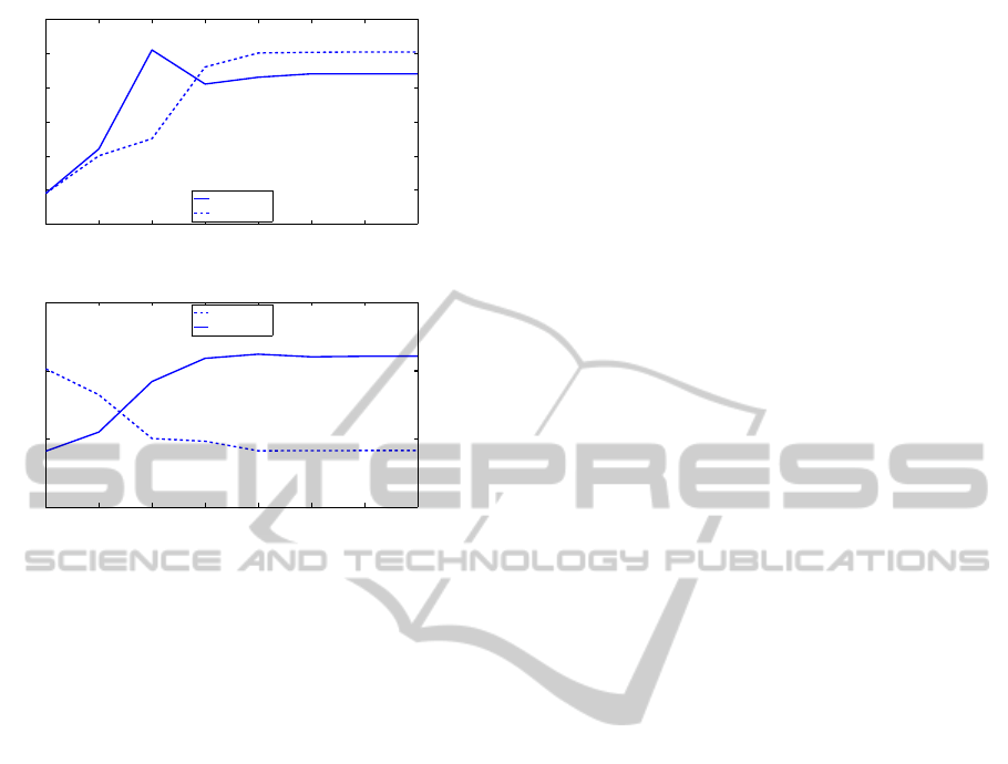
The number of observation points N

has marginal

effects on the speed and accuracy of the method. In

Fig. 5(a) and Fig. 5(b) magnitude and phase of the op-

timized R

and R

for structure of Fig. 4 (described

Table 3: Reﬂection coefﬁcients for structure shown in Fig. 1

with n

= 5.477, n

= 1, t = 0.19λ, w = 2λ, N

= 200.

CGF-RFFM IE-MoM

-optimization (Parsa and Paknys, 2007b)

-0.263+j0.654 -0.263+j0.752

0.443+j0.758 0.443+j0.759

0.315+j0.841 0.315+j.841

Time < 8 sec > 6 min

Figure 4: Three layer truncated dielectric slab waveguide.

in Table 4) are depicted for N

. Good convergence

can be seen in the optimized reﬂection coefﬁcients,

by increasing N

5 CONCLUSION

A novel method for reﬂection of guided mode at the

end-facet of optical waveguide is presented. The

method is based on the formulation of characteris-

tics Green’s function which is combined with rational

function ﬁtting method. In the closed-form derivation

for spatial Green’s function of ﬁnite dielectric slab

waveguide, discrete and continuous spectrum contri-

bution are expressed in appropriate forms which can

be imported in optimization problem to obtain an ex-

act reﬂection coefﬁcients of guided modes. The main

CombinationofCharacteristicGreen'sFunctionTechniqueandRationalFunctionFittingMethodforComputationof

ModalReflectivityattheOpticalWaveguideEnd-facet

50 100 150 200 250 300 350 400

0.3

0.31

0.32

0.33

0.34

0.35

0.36

Magnitude

50 100 150 200 250 300 350 400

0.49

0.5

0.51

0.52

0.53

0.54

0.55

Phase (rad)

Magnitude

Phase

(a)

50 100 150 200 250 300 350 400

0.65

0.7

0.75

0.8

Magnitude

50 100 150 200 250 300 350 400

0.1

0.15

0.2

0.25

Phase (rad)

Phase

Magnitude

(b)

Figure 5: Convergence of magnitude and phase of opti-

mized a) R

and b) R

, for different N

for structure of

Table 4.

advantages of this method lie in its rapidity as well

as accuracy. By using COMSOL for exact results of

spatial Green’s function for optimization, total CPU-

time is much less than rigorous methods. In gen-

eral, for all planar multilayered waveguide the for-

mulation can be easily derived for all components of

dyadic Green’s function to have reﬂection coefﬁcients

of guided modes at the end-facet of truncation.

REFERENCES

Chen, Y., Lai, Y., Chong, T. C., and Ho, S.-T. (2012). Exact

solution of facet reﬂections for guided modes in high-

refractive-index-contrast sub-wavelength waveguide

via a fourier analysis and perturbative series summa-

tion: Derivation and applications. J. Lightw. Technol.,

30(15):2455–2471.

Coleman, T. F. and Li, Y. (1996). An interior trust region ap-

proach for nonlinear minimization subject to bounds.

SIAM journal on optimization, 6(2):418–445.

Derudder, H., Olyslager, F., De Zutter, D., and van den

Berghe, S. (2001). Efﬁcient mode-matching analysis

of discontinuities in ﬁnite planar substrates using per-

fectly matched layers. IEEE Trans. Antennas Propag.,

49(2):185 –195.

El-Refaei, H., Betty, I., and Yevick, D. (2000). The appli-

cation of complex Pade approximants to reﬂection at

optical waveguide facets. IEEE Photon. Technol. Lett.,

12(2):158–160.

Faraji-Dana, R. (1993a). An Efﬁcient and Accurate Green’s

Function Analysis of Packaged Microwave Integrated

Circuits. Thesis (Ph.D.)–University of Waterloo.

Faraji-Dana, R. (1993b). An Efﬁcient and Accurate Green’s

Function Analysis of Packaged Microwave Integrated

Circuits. Thesis (Ph.D.)–University of Waterloo.

Gelin, P., Petenzi, M., and Citerne, J. (1981). Rigorous anal-

ysis of the scattering of surface waves in an abruptly

ended slab dielectric waveguide. IEEE Trans. Microw.

Theory Techn., 29(2):107 – 114.

Hardy, A. (1984). Formulation of two-dimensional

reﬂectivity calculations for transverse-magnetic-like

modes. J. Opt. Soc. Am. A., 1(7):760–763.

Hua, Y. and Sarkar, T. (1989). Generalized pencil-of-

function method for extracting poles of an EM sys-

tem from its transient response. IEEE Trans. Antennas

Propag., 37(2):229 –234.

Ikegami, T. (1972). Reﬂectivity of mode at facet and oscil-

lation mode in double-heterostructure injection lasers.

IEEE J. Quantum Electron., 8(6):470–476.

Jamid, H. and Khan, M. (2007). 3-D full-vectorial anal-

ysis of strong optical waveguide discontinuities us-

ing Pade approximants. IEEE J. Quantum Electron.,

43(4):343–349.

Lewin, L. (1975). A method for the calculation of the

radiation-pattern and mode-conversion properties of a

solid-state heterojunction laser. IEEE Trans. Microw.

Theory Techn., 23(7):576–585.

Michalski, K. and Mosig, J. (1997). Multilayered media

Green’s functions in integral equation formulations.

IEEE Trans. Antennas Propagat., 45(3):508 –519.

Parsa, A. and Paknys, R. (2007a). Interior Green’s function

solution for a thick and ﬁnite dielectric slab. IEEE

Trans. Antennas Propag., 55(12):3504 –3514.

Parsa, A. and Paknys, R. (2007b). Interior Green’s function

solution for a thick and ﬁnite dielectric slab. IEEE

Trans. Antennas Propag., 55(12):3504 –3514.

Rozzi, T. and Veld, G. (1980). Variational treatment of the

diffraction at the facet of d.h. lasers and of dielectric

millimeter wave antennas. IEEE Trans. Microw. The-

ory Techn., 28(2):61–73.

Shishegar, A. A. and Faraji-Dana, R. (2003). A closed-form

spatial Green’s function for ﬁnite dielectric structures.

Electromagnetics, 23(7):579–594.

Torabi, A., Shishegar, A. A., and Faraji-Dana, R. (2013).

Application of the characteristic Green’s function

technique in closed-form derivation of spatial Green’s

function of ﬁnite dielectric structures. In Compu-

tational Electromagnetics Workshop (CEM), 2013,

pages 54–55.

Torabi, A., Shishegar, A. A., and Faraji-Dana, R. (2014a).

Analysis of modal reﬂectivity of optical waveguide

end-facets by the characteristic Green’s function tech-

nique. J. Lightw. Technol., 32(6):1168–1176.

Torabi, A., Shishegar, A. A., and Faraji-Dana, R. (2014b).

An efﬁcient closed-form derivation of spatial Green’s

function for ﬁnite dielectric structures using character-

istic Green’s function-rational function ﬁtting method.

IEEE Trans. Antennas Propagat., 62(3).

PHOTOPTICS2015-InternationalConferenceonPhotonics,OpticsandLaserTechnology

Wei, S.H. and Lu, Y. Y. (2002). Application of Bi-CGSTAB

to waveguide discontinuity problems. IEEE Photon.

Technol. Lett., 14(5):645–647.

Yevick, D., Bardyszewski, W., Hermansson, B., and Glas-

ner, M. (1991). Split-operator electric ﬁeld reﬂection

techniques. IEEE Photon. Technol. Lett., 3(6):527–

529.

Yevick, D., Bardyszewski, W., Hermansson, B., and Glas-

ner, M. (1992). Lanczos reduction techniques for elec-

tric ﬁeld reﬂection. J. Lightw. Technol., 10(9):1234–

1237.

Yu, C. and Yevick, D. (1997). Application of the bidirec-

tional parabolic equation method to optical waveguide

facets. J. Opt. Soc. Am. A., 14(7):1448–1450.

CombinationofCharacteristicGreen'sFunctionTechniqueandRationalFunctionFittingMethodforComputationof

ModalReflectivityattheOpticalWaveguideEnd-facet