
Measuring Distance by Angular Domain Filtering
Wei-Jun Chen
Systemtechnik, Carl Zeiss Meditec AG, G
¨
oschwitzer Straße 51–52, 07745, Jena, Germany
Keywords:
Angular Domain filtering, Afocal System, Transform, Distance measurement, Bi-lateral telecentric optics.
Abstract:
In this paper a paraxial imaging system with incoherent illumination is interpreted as a signal processing
system in which a thin lens performs a forward angular transform on light rays traveling through it. Inverse
angular transform exists and could be performed by another thin lens which coincides its focus plane with the
first. The common focus plane acts as an angular domain, on which filtering is possible by placing aperture
stops. A symmetrically angular filtering results in a direct correspondence between a recorded signal and its
object distance. Such a “transform–filtering–inverse transform” system could be understood as a modified
tele–centric system, with which a novel concept for measuring a distance without focusing on the target is
suggested.
1 INTRODUCTION
Although an imaging system is generally considered
as the data supplier of a signal processing system,
there is no limit to extend processing concepts cov-
ering data acquisition. In Fourier optics (Goodman,
1968), concepts including Fourier transform, fre-
quency domain filtering, point spread function (PSF),
etc. are employed to get deep understanding of a thin–
lens system. Such an understanding plays a key role
in improving image quality in a wide range of imag-
ing fields like bio–medical imaging, astronomy, and
also electron microscopy.
On another hand, the meaning of high im-
age quality is much more than just amusing hu-
man eyes. In photometry high image quality often
means enhanced landmarks and ignorable environ-
ment, while in medical diagnosis high image qual-
ity normally asks for high signal–to–noise ratio for
disease symptoms where misleading message is not
acceptable. To satisfy various image quality require-
ments, many specified optical designs have been pro-
posed in past decades. As an example, tele–centric
optics (Lenhardt, 2001), is specially designed for high
precision and distance invariant measuring system.
Illuminated with incoherent light, an imaging pro-
cess could be generally described as a ray traveling
process: light rays are emitted from object points; af-
terward they freely travel in air; thin lenses collect
such rays and change their directions targeting a dig-
ital sensor; finally the sensor records the energy car-
ried by these rays as pixel intensities.
In the same direction of Fourier optics, this paper
tries to interpret such an incoherence ray journey by
signal processing terms, where a transform, namely
as angular transform, and its inverse are defined to
describe the ray mapping between two focus planes
of a thin lens. All the rays with the same traveling
direction from a thin lens’ anterior focus plane, will
travel through an unique position on its posterior fo-
cus plane, and vice versa. If two thin lenses are so
placed that the second lens coincides its anterior focus
plane with the first lens’ posterior focus plane, like a
4–f system in Fourier optics or an afocal system in
telescopy, selecting rays by their directions could be
fulfilled by placing filters on the angular domain, i.e.,
the common focus plane. Moreover, when a single–
hole aperture stop is placed at the angular domain cen-
ter, a standard bi–lateral tele–centric system is built.
It is asked, that if the aperture stop is not placed at
the domain center, i.e., performing an off–axis angu-
lar filtering, what result should be obtained? Section 4
gives out an answer that by off–axis angular filtering,
object distance could be measured by single snapshot
imaging.
The rest of this paper is organized as following:
in next section some further readings are suggested
for more background information; Section 3 describes
the angular transform, its inverse, and the angular
domain in details; Section 4 introduces the concept
of measuring distance by angular domain filtering,
which is further demonstrated by an imaging experi-
85
Chen W..
Measuring Distance by Angular Domain Filtering.
DOI: 10.5220/0005336400850090
In Proceedings of the 3rd International Conference on Photonics, Optics and Laser Technology (PHOTOPTICS-2015), pages 85-90
ISBN: 978-989-758-092-5
Copyright
c
2015 SCITEPRESS (Science and Technology Publications, Lda.)
ment in Section 5; Afterward Section 6 provides some
conceptual discussions; Finally Section 7 concludes
this paper with a brief discussion on future works and
open questions.
2 FURTHER READINGS
Along with the rapid development of digital sensor
techniques, kinds of optical systems have been de-
signed for digital imaging based machine vision ap-
plications (Zeuch, 2000) (Jaehne and ecker, 2000),
where tele–centric optics plays an important role for
focus analysis (Watanabe and Nayar, 1997), non–
contact velocity sensing (Berger, 2002) and 3D imag-
ing (Djidel et al., 2006) (Kim and Kanade, 2011). Ge-
ometric optics, which provides the design disciplines
for imaging optics, is normally based on the paraxial
approximation, which is often described by the ma-
trix method (Gerrard and Burch, 2012) in a simple
but powerful way.
3 ANGULAR TRANSFORM
A light ray traveling in an imaging system could
always be described by a 5–dimensional vector:
(x,y,z,α,β), where (x, y,z) denotes a spatial position
in a Cartesian coordinate system
1
, and (α, β) denotes
two angles describing the ray direction~r =~r
x
+~r
y
+~r
z
,
where~r
x
,~r
y
and~r
z
denote three axis projections of ~r.
Without loss of generality, α denotes the angle be-
tween ~r and ~r
z
, and β denotes the angle between ~r
x
and~r
x
+~r
y
, as shown in Fig. 1.
Figure 1: A traveling ray~r, its axis projections of~r
x
,~r
y
,~r
z
,
and its direction angles (α,β).
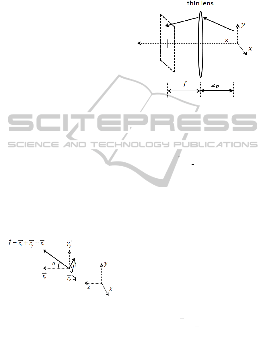
Placing a thin lens perpendicular to the z axis, a
ray traveling through it will arrive at a spatial position
on its posterior focus plane, as shown in Fig. 2.
The thin lens performs a transform on a given
light ray (x,y,z, α, β). Defining c = tanα cos β and
1
In this paper the right-hand rule is applied for defining
a 3–dimensional Cartesian coordinate system.
Figure 2: A light ray traveling through a thin lens, where f
denotes the lens’ focus length.
s = tanα sin β, such a transform could be expressed
as:
x
f
y
f
c
f
s
f
=
0 0 f 0
0 0 0 f
−
1
f
0 1 0
0 −
1
f
0 1
x + z
p
c
y + z
p
s
c
s
, (1)
where z
p
denotes the z–axis projection of a traveling
path from its starting position z to the thin lens posi-
tion z
lens
: z
p
= z
lens
− z.
The 4 × 4 transform matrix in Eq. 1 is a combina-
tion of two element transform matrices (Gerrard and
Burch, 2012): one for free space light propagation
and another one for thin lens with focus length of f .
The vector (x
f
,y
f
,c
f
,s
f
) defines a light ray passing
through the spatial position ((x
f
,y
f
,z
f
) on the back
focus plane (i.e., z
f
= z
lens
+ f ), with its direction
defined by (c
f
,s
f
). Since the following equation ex-
ists:
1 0 − f 0
0 1 0 − f
1
f
0 0 0
0
1
f
0 0
0 0 f 0
0 0 0 f
−
1
f
0 1 0
0 −
1
f
0 1
= I, (2)
an inverse transform could be defined:
x
v
y
v
c
v
s
v
=
1 0 f
v
0
0 1 0 f
v
−
1
f
v
0 0 0
0 −
1
f
v
0 0
x
f
y
f
c
f
s
f
, (3)
where the sign difference in Eq. 2 and 3 indicates two
different light traveling directions: in Eq. 2 a ray goes
backward and in Eq. 3 a ray goes forward. Physically
Eq. 3 is equivalent to placing another thin lens with
PHOTOPTICS2015-InternationalConferenceonPhotonics,OpticsandLaserTechnology
86
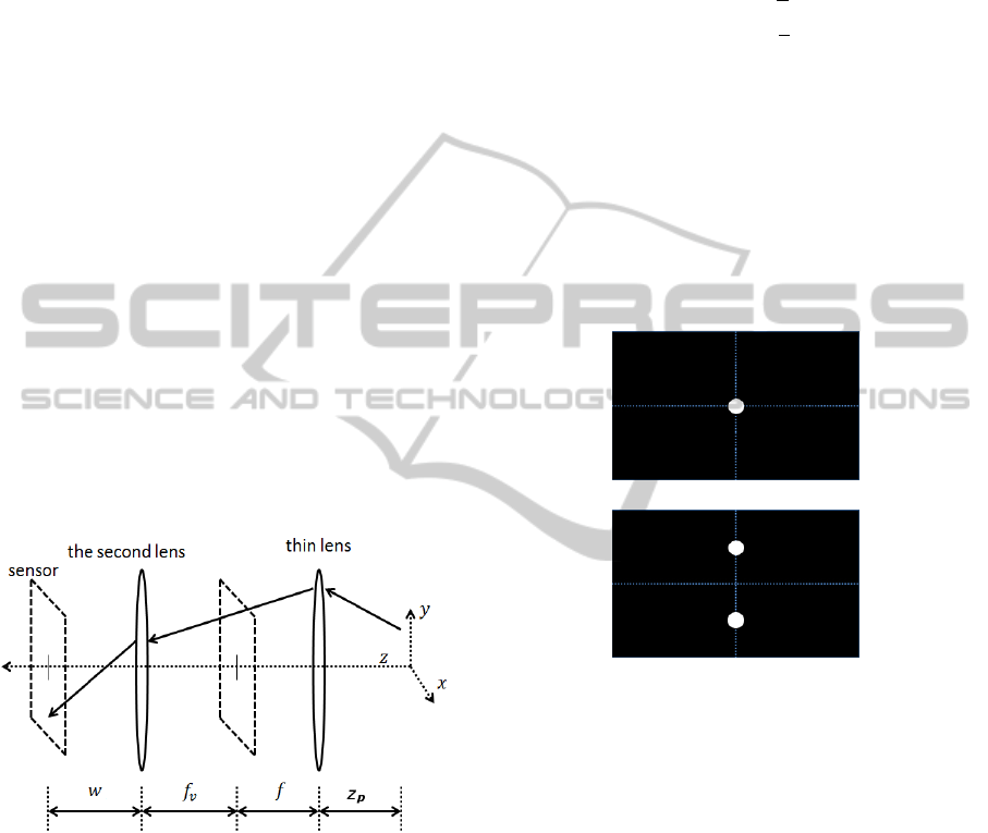
focus length f
v
after the first one, with a distance f +
f
v
thus that the rear lens coincides its focus plane with
the front lens. The above inverse transform results
in a new ray just traveling through the second lens.
Placing a sensor after the second lens with a distance
w, as shown in Fig. 3, the light ray will finally be
recorded at a 2D sensor position, where we have
x
i
y
i
c
i
s
i
=
1 0 w 0
0 1 0 w
0 0 1 0
0 0 0 1
x
v
y
v
c
v
s
v
. (4)
Angular Transform: Above Eq. 1–4 describe a ray
journey in which a signal is emitted from a spatial po-
sition (x, y,z) and finally is recorded by a 2D sensor at
(x
i
,y
i
). Between signal emission and recording, a for-
ward transform and its inverse are performed sequen-
tially by two thin lenses. On the transform domain,
each signal, i.e., each light ray, travels through a 2D
spatial position (x
f
,y
f
) which only depends on the
angular information of the signal and is independent
to its z position. Such a transform is named as angu-
lar transform while each 2D position on the common
focus plane, namely as the angular domain, is equiv-
alent to a unique (α,β) pair describing the angular
information of rays.
Figure 3: The second lens with focus length of f
v
coincides
its focus plane with the first lens, and a sensor after it with
a distance of w.
4 DISTANCE FROM ANGULAR
FILTERING
Although a light ray in Eq. 4 is finally recorded by a
2D sensor, the z information of its origin is still pre-
served. Defining m = ( f / f
v
), we have:
z
p
= m( f + f
v
) − m
2
w − m × x
i
/c − x/c, (5)
z
p
= m( f + f
v
) − m
2
w − m × y
i
/s − y/s. (6)
Moreover, if two rays with symmetry angles,
i.e., (±α,β) emitted from the same 3D source are
recorded, the z information could be obtained by mea-
suring a distance between two sensor positions:
z
p
= m( f + f
v
) − m
2
w −
m
2
(x
α
i
− x
−α
i
)/c, (7)
z
p
= m( f + f
v
) − m
2
w −
m
2
(y
α
i
− y
−α
i
)/s, (8)
where (x
α
i
,y
α
i
) denotes the sensor position of the light
ray (α,β), as well as (x
−α
i
,y
−α
i
) for the light ray
(−α,β).
The selective ray recording for Eq. 7 and 8 could
be fulfilled by placing a filter on the angular domain.
An example for such a filter is shown in Fig. 4(b),
where two small holes are symmetrically defined with
a distance h from the domain center, allowing light
rays with angle of (α = ±tan
−1
(h/ f ),β = 90
◦
) to be
finally recorded.
(a)
(b)
Figure 4: Two example filters for angular domain filtering:
a), a near–zero–pass filter; b), a symmetrically off–axis
filter. Both of them are thin (0.1 mm thickness) aluminum
sheets with small holes φ 1.5 mm.
5 EXPERIMENT
An imaging experiment has been performed for a
conceptual demonstration for above angular domain
filtering. An eLED torch for kids (Fig. 5(a)), inside
which a LED lamp is fixed at the center of a cone
base, and the inner cone surface is tiled with small
mirrors (Fig. 5(b)), was adopted as our object light
source.
This object, a consumer CMOS sensor, and two
thin lenses (with the same focus lenth of 75 mm) were
placed in the way described in Fig. 3. Without sur-
prise, for a fixed sensor position, roughly two focused
object images could be observed with different object
MeasuringDistancebyAngularDomainFiltering
87
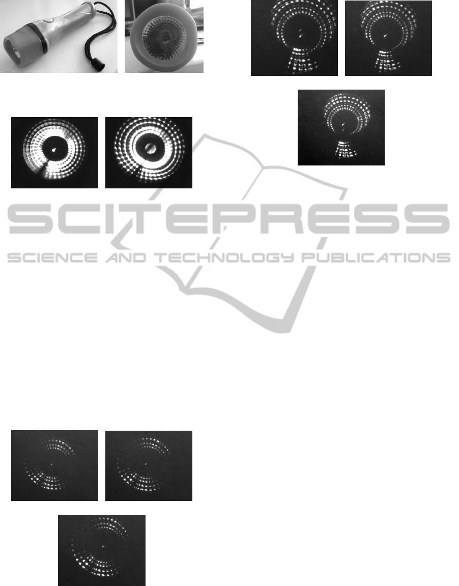
(a) (b)
Figure 5: The object light source: a), an eLED torch for
kids; b), its front view.
(a) (b)
Figure 6: Two conjugate images of the light source: a), the
sharp lamp spot (center) and the surrounding blurred virtual
lamps; b), the blurred lamp spot and sharp virtual lamps.
positions: one for the center LED lamp, and another
one for the virtual lamp images generated from mirror
reflection, as shown in Fig. 6
A near–zero–pass angular domain filtering has
been performed in the experiment. Images were
recorded from three different object positions: fo-
cusing on the virtual lamp, focusing on the center
real LED lamp, and the third one further than these
two focusing positions. As shown in Fig. 7, all the
recorded images contain sharp signals and are similar
to each other with the help of near–zero–pass angular
filtering.
Applying the example filter described in Fig. 4(b),
an off–axis angular domain filtering has also been
(a) (b)
(c)
Figure 7: Imaging results from a near–zero–pass angular
filtering, at different object positions: a), focusing position
of the virtual lamp signal ; b), focusing position of the LED
lamp; c), an object position further than a) and b).
(a) (b)
(c)
Figure 8: Imaging results from an off–axis angular filtering,
at different object positions: a), focusing position of the vir-
tual lamp signal ; b), focusing position of the LED lamp; c),
an object position further than a) and b).
performed. Images were recorded at the same three
positions as above. When the object is placed at the
focusing position of the center lamp, only one spot
was recorded in the image center (Fig.8(b)); Oth-
erwise two vertically separated spots were recorded
(Fig.8(a)8(c)).
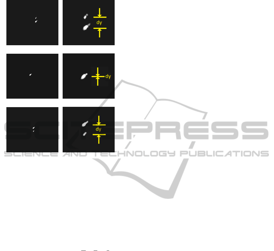
Based on the recorded images in Fig.8, basic dig-
ital image processing techniques were further em-
ployed to measure the corresponding object distances.
The center LED signals were picked out and en-
hanced (Fig.9(a), 9(c) and 9(e)); Gravity centers of
individual spots were detected from the enhanced im-
ages; Afterwards for each image, the lateral distance
between two gravity centers of separated spots was
measured. In above experiment, three lateral dis-
tances were measured: dy > 0 for Fig.9(b), dy = 0
for Fig.9(d) and dy < 0 for Fig.9(f), where dy denotes
the vertical distance of y
α
i
− y
−α
i
; Finally the three
object distances for this experiment were calculated
from Eq.8 based on the measured lateral distances of
dy, and the system design parameters including the
sensor position w, the filter parameter s, and two lens
parameters f and f
v
.
6 DISCUSSIONS
In this section, the concept of measuring distance by
angular filtering will be discussed in three concep-
tual directions: 1), distance from an afocal system;
2), transform by a thin lens; 3), off–axis tele–centric
system.
PHOTOPTICS2015-InternationalConferenceonPhotonics,OpticsandLaserTechnology
88
(a) (b)
(c) (d)
(e) (f)
Figure 9: Measurements from an off–axis angular filtering,
at different object positions: a) and b), focusing position
of the virtual lamp signal ; c) and d), focusing position of
the LED lamp; e) and f), an object position further than
a) and b). The image b) is a magnified version for better
visualization of a), as well as the image d) for c) and image
f) for e).
6.1 Distance from an Afocal System
Retrieving object distance from camera parameters
has been addressed for a long time. A direct way
is based on the thin lens equation
1
d
o
+
1
d
i
=
1
f
, from
which the object distance d
o
could be directly calcu-
lated from the imaging distance d
i
and the lens’ focus
length f , with the condition that the image is well fo-
cused.
Considering that the two thin lenses in Fig. 3
work actually as one thin lens with a compound focus
length of ∞, say, an afocal lens (Greivenkamp, 2004),
the distance relationship between the object and its
conjugate image is simplified as:
z
p
= m( f + f
v
) − m
2
w, (9)
from which angular separations, x
α
i
−x
−α
i
in Eq. 7 and
y
α
i
− y
−α
i
in Eq. 8, are equal to zero.
Without finely searching for its corresponding
conjugate of a measured object in either a focusing
system, or an afocal system, this paper suggests to
measure its axial distance, i.e., z
p
= z
lens
− z, by mea-
suring its spatial separation defined by an angular
domain filter, where the image distance w is fixed
but could also be varied thus that introducing more
flexibility for system design.
6.2 Transform by a Thin Lens
In spite of its wave optics nature, Fourier optics could
also be explained by geometric optics (Jutamulia and
Asakura, 2002). Physically an above afocal system
has the same lens layout as a 4– f system in Fourier
optics. Normal imaging systems are generally based
on non–coherent illumination while Fourier optics is
based on coherent light. With a thin lens, the su-
perposition principle works on the real field resulting
in an angular domain for non–coherent rays, while it
works on the complex field resulting in a spatial fre-
quency domain for coherent rays. In both situations
the transform performed by a thin lens decomposes a
source signal in a particular domain, on which filters
select preferred components for further signal record-
ing. As shown in Eq. 7 and 8, angular domain filtering
provides an opportunity to measure an object’s axial
position by measuring one 2D distance on its image,
which might be either in–focused or out–focused.
6.3 Off–axis Tele–centric Optics
If an aperture stop of a single hole is placed at the
angular domain center, only the light rays with near–
zero angles, i.e., ∀β,|α| ≈ 0, will arrive in the sen-
sor. All the recorded light rays are parallel to the op-
tical axis; Such an optical system is a bi–lateral tele–
centric system.
It is widely understood that a tele–centric imaging
system provides more accuracy and better repeata-
bility for image based measurements, which are ex-
pected to be theoretically invariant to the object dis-
tance because of the parallel–to–axis nature of re-
ceived signals. This paper further interprets a tele–
centric system as a zero–angle–pass filtering system.
Moreover, once the aperture stop is shifted from the
domain center, signals with other angles of α,β will
be selected, where the allowing angles are defined by
the spatial 2D position of the aperture stop. Two sym-
metrically placed filtering holes make it possible to
measure the axial position of an object with or with-
out focusing on it.
7 CONCLUSION AND FUTURE
WORKS
This paper is based on a general optical sys-
tem, which appears as the afocal system in tele-
MeasuringDistancebyAngularDomainFiltering
89

scope (Greivenkamp, 2004), the bi–lateral tele–
centric imaging system in photometry (Lenhardt,
2001), as well as the 4–f correlation system in Fourier
optics (Goodman, 1968). In principle all these sys-
tems use the same lens layout: two thin lenses with a
common focus plane. Such a lens layout appears also
in many specified applications like Schlieren photog-
raphy (Settles, 2001) in which the concept of angular
domain filtering is implicitly employed.
It is well known that with coherence light il-
lumination, the common focus plane of the above
two–lens–layout, is a Fourier domain (Goodman,
1968) (Jutamulia and Asakura, 2002). This paper
further explicitly points out that, for incoherent light,
the common focus plane is NOT Fourier domain any
more, but an angular domain. In this paper a set of
4 × 4 matrix equations (Eq. 1–4) explicitly describe
the forward transform, the domain, as well as the in-
verse transform.
Based on the above transform interpretation of
thin lenses, it is possible to select and exclude infor-
mation according to its incoming angle. Particularly
selecting the near–zero–angle lights, i.e., placing a
small–aperture stop at the center of the common focus
plane (Fig. 4(a)), the system is a bilateral tele–centric
system.
This paper further points out that, shifting the
small aperture stop away from the domain center re-
sults in non–zero angular domain filtering. Espe-
cially, if two symmetrically angular filtering holes are
used (Fig.4b), the object distance could be measured
from an one–shot image, based on Eq. 7, 8, and 9.
It is not a surprise that an afocal image with finite
opening mask contains information about the object
distance. But to retrieval such distance information
often needs to analyze blurred 2D images. In this
paper the distance information is directly calculated
from lateral separation of sharp signals, rather than
analyzing blur information from input data.
Some questions are still open for future works. At
first, the experiment described in this paper is a quali-
tative one. More experiments should be performed for
quantitative evaluations like the object defocus ampli-
tude, measurement resolution, as well as the system
error function; Second, this paper is limited to the
same scale of geometric optics based on the paraxial
approximation. The measuring accuracy of an object
distance in Eq. 7 and 8 should be further evaluated
since there is a gap between the physical reality and
mathematical models. For instance, the zero–angle–
pass filter in a tele–centric system has a finite aperture
size so that recorded signals are “parallel enough” to
the optical axis rather than strictly “parallel” to it.
Such a gap should also be further addressed for ac-
curacy evaluation; Third, a filter placed in the angular
domain does not only select and exclude signals ac-
cording to its domain position as well as its aperture
shape, but also heavily reduce the energy projected
on the sensor. Digital signal enhancement and ob-
ject detection from a weak energy image should be
also taken into account for designing angular domain
filtering systems.
ACKNOWLEDGEMENT
The author would like to thank Dr. Hexin Wang,
Dr. Christopher Weth, Dr. Matthias Reich, Mr. Ralf
Ebersbach, and other anonymous reviewers for their
valuable suggestions.
REFERENCES
Berger, C. (2002). Design of telecentric imaging systems
for noncontact velocity sensors. Optical Engineering,
41(10):2599–2606.
Djidel, S., Gansel, J. K., Campbell, H. I., and Greenaway,
A. H. (2006). High-speed, 3-dimensional, telecentric
imaging. Optical Express, 14(18):8269–8277.
Gerrard, A. and Burch, J. M. (2012). Introduction to Matrix
Methods in Optics. Dover Publications, Incorporated.
Goodman, J. W. (1968). Introduction to Fourier Optics.
McGraw-Hill, New York.
Greivenkamp, J. E. (2004). Field guide to geometrical op-
tics. SPIE Press, Bellingham, WA.
Jaehne, E. and ecker, H. H. (2000). Computer Vision and
Applications: A Guide for Students and Practitioners.
Academic Press.
Jutamulia, S. and Asakura, T. (2002). Optical fouier-
transform theory based on geometrical optics. Optical
Engineering, 41(01):13–16.
Kim, J.-S. and Kanade, T. (2011). Multiaperture tele-
centric lens for 3d reconstruction. Optics Letters,
36(7):1050–1052.
Lenhardt, K. (2001). Optical measurement techniques
with telecentric lenses. In Know How: Technical
and Scientific Contributions, pages 1–61. Schneider
Kreuznach.
Settles, G. S. (2001). Schlieren and shadowgraph tech-
niques: Visualizing phenomena in transparent media.
Springer-Verlag, Berlin.
Watanabe, M. and Nayar, S. K. (1997). Telecentric op-
tics for focus analysis. IEEE Trans. on PAMI,
19(12):1360–1365.
Zeuch, N. (2000). Understanding and Applying Machine
Vision, Second Edition, Revised and Expanded. CRC
Press.
PHOTOPTICS2015-InternationalConferenceonPhotonics,OpticsandLaserTechnology
90
