
Face Recognition by Fast and Stable Bi-dimensional Empirical Mode
Decomposition
Esteve Gallego-Jutglà
1
, Saad Al-Baddai
2
, Karema Al-Subari
2
, Ana Maria Tomé
3
,
Elmar W. Lang
2
and Jordi Solé-Casals
1
1
Data and Signal Processing Group, University of Vic, Central University of Catalonia, Sagrada Família 7,
08500 Vic, Spain
2
Institute of Biophysics, University of Regensburg, 93040 Regensburg, Germany
3
IEETA, DETI, University of Aveiro, 3810-193 Aveiro, Portugal
Ke
ywords: Face Recognition, Fast and Stable Bi-dimensional Empirical Mode Decomposition, Linear Discriminant
Analysis, Biometrics.
Abstract: In this study the use of a new fast and stable decomposition technique, bi-dimensional empirical mode
decomposition, is used for face recognition tasks. Images are decomposed individually, and then the
distance with reference images is computed. Three different types of distances are tested. Then class
association is based on minimum distance and by using a classifier. Preliminary results (90.0% of
classification rate) are satisfactory and will justify a deep investigation on how to apply this bi- dimensional
decomposition technique for face recognition.
1 INTRODUCTION
Face recognition is a field of study that has been
developed in recent years. Errors of classification in
this field of study have decreased over the last
twenty years by three orders of magnitude when
recognizing frontal faces (Phillips et al. 2011). Face
recognition has been developing quickly, and it
seems that there is not a limit for the capacity of this
system, because the data entry of these systems can
be really big. For this reason, researchers aim to
improve face recognition systems by introducing
new characteristics and new working lines that can
be valid for the development of these kinds of
systems (Iancu et al. 2007).
Usually applications given to this field are as
diverse as an online search for images or the use of
face recognition for security (Wagner et al. 2012).
Different examples of commercial software that use
face recognition are Picassa, iPhoto or Windows
Live Gallery. On the other hand, several security
laws have been proposed in order to increase control
access to different places. Therefore face recognition
has been used in continuous monitoring or access
security (Woodward et al. 2002; Xiao 2007).
This paper explores a promising strategy for face
recognition, using a new decomposition technique,
called Fast and Stable Bi-dimensional Empirical
Mode Decomposition (FSBEMD). Images of the
subjects are decomposed and compared before the
classification is performed. Previous work (Gallego-
Jutglà et al. 2013) studied the use of Multivariate
Empirical Mode Decomposition (mEMD) for the
same purpose. However, in that approach only the
information contained in one dimension was
evaluated due to the unfolding of the images before
the computation of mEMD. In this new approach,
FSBEMD is computed with images in the original
format, without unfolding. Therefore the information
contained in the two dimensions of the image is
taken into account for classification.
This paper is organized as follows: After this
introduction, methods are detailed in Section 2,
including the explanation of the data base, the
FSBEMD technique and the signal processing
applied to the data. Results of applying these
methods on the images are presented in Section 3.
Finally, Section 4 is devoted to discussion of the
obtained results and to present conclusions and
future lines of research.
385
Gallego-Jutglà E., Al-Baddai S., Al-Subari K., Maria Tomé A., Lang E. and Solé-Casals J..
Face Recognition by Fast and Stable Bi-dimensional Empirical Mode Decomposition.
DOI: 10.5220/0005337003850391
In Proceedings of the International Conference on Bio-inspired Systems and Signal Processing (MPBS-2015), pages 385-391
ISBN: 978-989-758-069-7
Copyright
c
2015 SCITEPRESS (Science and Technology Publications, Lda.)
2 METHODS
Methods used to compute the image classification
using FSBEMD are detailed in this section. First in
Section 2.1 the used data base is presented. In
Section 2.2 an introduction to Bi-dimensional
Empirical Mode Decomposition (BEMD) is
presented and then in Section 2.3 FSBEMD is
detailed. Section 2.4 explains the classification
system used to compute image classification and
cross-validation. Finally in Section 2.5 the image
processing applied is detailed by jointly using all the
methods presented before.
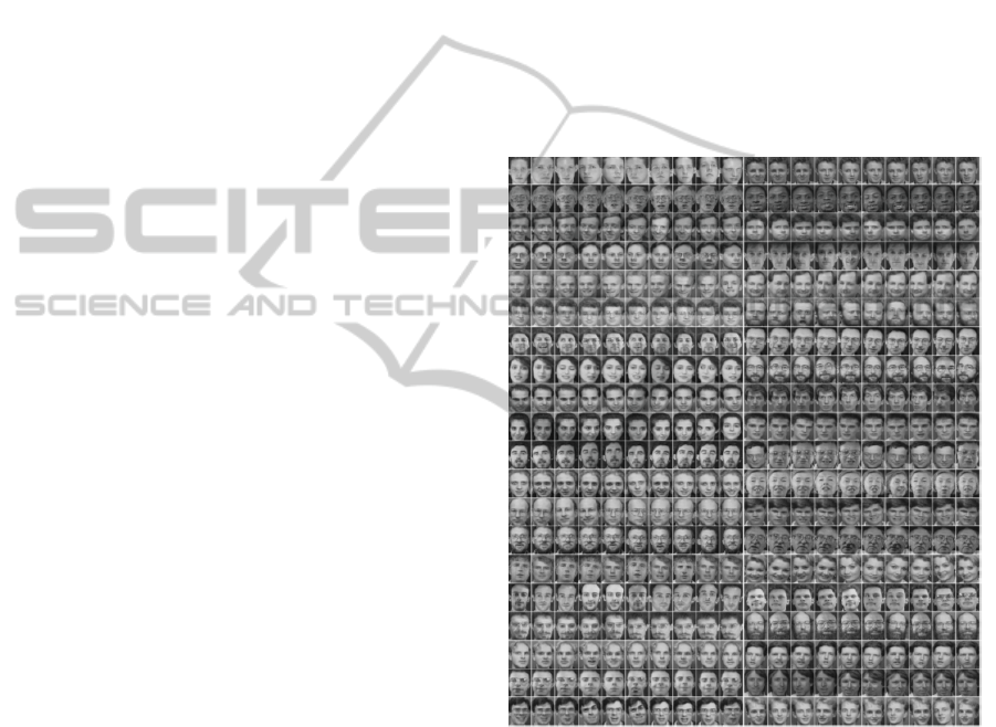
2.1 Data Base
The used data base contains 10 different images for
40 different subjects. Therefore a total of 400
different images are contained in the data base.
Images were taken with a dark background, with
frontal position and with different orientations of the
subjects.
This data base presents images with different
gestural positions, such as eyes open, eyes closed,
smile or no smile, glasses or no glasses and
illumination variations. The illumination variations
are not defined. All images are grey scale of 256
values, with a size of 92 x 112 pixels. The whole
dataset is presented in Figure 1.
2.2 Bi-dimensional Empirical Mode
Decomposition
Empirical Mode Decomposition (EMD) or BEMD is
a sifting process that decomposes a signal into its
Intrinsic Mode Functions (IMFs) or Bi-dimensional
Intrinsic Mode Functions (BIMFs) and a residue
based basically on the local frequency or oscillation
information.
The first IMF/BIMF contains the highest local
frequencies of oscillation or the smallest local spatial
scales, the final IMF/BIMF contains the lowest local
frequencies of oscillation and the residue contains
the trend of the signal/data. Like time frequency
distribution with EMD, acquiring the space spatial-
frequency distribution of 2D data/image is possible
with BEMD, which may be named as Bi-
dimensional Hilbert Huang Transform (BHHT).
2.2.1 General BEMD
General BEMD is a sifting process that decomposes
Xm,n into multiple hierarchical components
known as BIMFs. A typical sifting process is
summarized in the following iterations:
i. Initialization: set, ,.
Identify all local maxima and local minima
of,.
ii. Interpolate the local maxima,
,,
to obtain the upper surface and local
minima,
,, to obtain the lower
surface.
iii. The mean ,
,
,
/2 is computed and
subtracted from , to
obtain′, ,.
iv. Update , by′,. Repeat steps
(i.) to (iii.) until the stopping criterion is
met.
Figure 1: Data base ORL (Olivetti Research Laboratory).
2.3 Fast and Stable Bi-dimensional
Empirical Mode Decomposition
Similar to other BEMD techniques, the number of
BIMFs and their characteristics are highly dependent
on envelope estimation techniques in the sifting
process, on the methods to detect extrema, and on
stopping criteria during the iterations. In that sense,
and with the intention of overcoming the difficulty
in implementing BEMD via the application of
surface interpolation, a novel
approach is proposed
introducing a tension parameter to cope with surface
interpolation problems. It uses Green's functions for
BIOSIGNALS2015-InternationalConferenceonBio-inspiredSystemsandSignalProcessing
386

spline interpolation to estimate the upper and lower
surfaces. Including surface tension greatly improves
the stability of the method relative to gridding
without tension.
Based on the properties of the proposed
approach, it is considered a FSBEMD. The latter
differs from the standard BEMD algorithm basically
in the process of robustly estimating the upper and
lower surfaces, and in limiting the number of
iterations per BIMF to a few iterations only. Hence,
the FSBEMD is considered as an efficient algorithm
compared to other BEMD algorithms. The details of
extrema detection and surface formation of the
FSBEMD process are discussed in the following
section.
2.3.1 Extract of Local Extrema
Local extrema are points that have the largest or
smallest function value relative to their immediate
neighbours. Detection of local extrema means
finding the local maxima and minima from the given
data. The 2D region of local maxima is called a
maxima map and the 2D array of local minima is
called a minima map, respectively. Like BEMD, a
neighbouring window method is employed to find
local maxima and local minima during intermediate
steps of the sifting process for estimating a BIMF of
any source image. In this method, a data point/pixel
is considered as a local maximum (minimum), if its
value is strictly higher (lower) than all of its
neighbours.
Let
|1,.... be a set of local
minima (maxima) of an - dimensional 2D
matrix such that it exists a small (large) circle
around any such local optimal point
on which the
function value is never larger (smaller) than ,
at
. Local extrema occur only at critical points.
Let,
. If 0 at a critical
point, then the critical point
is a local extremum.
The signs of
and
determine whether the point
is a maximum or a minimum. If 0 at a critical
point, then the point
is saddle point. In practice,
a44 or 33 window results in an optimal
extrema map for a given 2D image. A 44
window is applied in this paper. However, a larger
window size might be used in some applications.
2.3.1 Green Function for Estimating
Surfaces
Spline interpolation, whether in one or two
dimensions, are basically used to find the smoothest
curve or surface that passes through a set of non-
uniformity data points. Green's functions are used to
shape an envelope or surface in terms of minimizing
the curvature of the envelope interpolating non-
uniformly spaced data points (Wessel & Bercovici
1998). The shape of the envelope or surface depends
on their tension parameter. So the Green's function
obeys the following relation (Wessel &
Bercovici 1998):
(1)
where,
and
are the bi-harmonic and
Laplace operators, respectively, is the flexural
rigidity of the curve or surface, is the tension used
at the boundaries, and
is the spatial position
vector. The equation above is solved by introducing
a new variable:
Ψ
(2)
Hence, Ψ
is the curvature of the Green's
function and (1) is rewritten as:
Ψ
Ψ
(3)
Then, the Fourier transform is taken:
Ψ
Ψ
1
(4)
Here, is the wavenumber vector and Ψ
is
the Fourier transform ofΨ
. In k-space, the
solution is:
Ψ
1
(5)
where
. Hence, the solution forΨ
could be obtained for any dimension. However, in
this paper we focus on the 2-D.
In the limit of a vanishing surface tension,
i.e. 0, or a diminished surface stiffness,
i.e. ⟶ 0, the Green's function behaves like
Ψ
|
|
log
|
|
or Ψ
log
|
|
,
respectively.
The general solution for this problem in a 2-D
spacial domain (Wessel & Bercovici 1998) can be
achieved by using Hankel transform as:
Ψ
1
1
|
|
||
(6)
where || represents the radial
wavenumber, and
is the adapted Bessel function
of the second kind and order zero. By plugging (6)
into (2) (with ||) we obtain:
1
r
|
|
(7)
Integrating the equation above two times results
in:
FaceRecognitionbyFastandStableBi-dimensionalEmpiricalModeDecomposition
387

|
|
|
|
(8)
is set from the condition
0 to
log
/
, and ignoring the common factor /
,
results in the final Green's function:
||
log||
(9)
Thus, the gradient of the Green's function is
1
|
|
||
|
|
(10)
Thus, by decreasing the tension parameter, the
solution is expected to reach the minimum curvature
solution (Sandwell 1987). In contrary, increasing the
tension parameter leads to an increase of
.
The trade-off between log
|
|
and
|
|
thus
achieves a continuous spectrum of Green's functions.
As → 0, we obtain the biharmonic Green's
function
log.
2.4 Classification
Extracted BIMFs, after applying FSBEMD to the
images, are first parameterized and then classified
using two different methods: by minimum distance
and by using Linear Discriminant Analysis (LDA).
2.4.1 Linear Discriminant Analysis
LDA is a well-known scheme for feature extraction
and dimension reduction. It has been used widely in
many applications involving high-dimensional data,
such as face recognition and image retrieval.
Classical LDA projects the data onto a lower-
dimensional vector space such that the ratio of the
between-class distances to the within-class distance
is maximized, achieving maximum discrimination
(Duda et al. 1995). The optimal projection
(transformation) can be readily computed by
applying the eigendecomposition on the scatter
matrices. See (Duda et al. 1995; Fukunaga 1990),
for details on the algorithm
2.4.2 Cross-validation for Classification
For the classification step, k-fold cross-validation is
used in order to ensure stable results. In this
evaluation methodology the original sample set is
randomly divided into subsets. Then, a single
subset is retained as the validation data for testing
the model, and the remaining 1 subsets are used
as training data. The cross-validation process is
repeated times, with each of the subsets used
exactly once as the validation data.
The obtained results from the folds are then
averaged in order to produce a single estimation.
The advantage of this method is that all observations
are used for both training and validation, and each
observation is used for validation exactly once. This
is the most robust evaluation method because it tries
to overcome a possible over-fitting. 10-fold cross-
validation is common, but with few samples only,
the leave-one-out cross-validation (LOOCV) could
be the best option.
LOOCV uses a single observation from the
original set as the validation data, and the remaining
observations as the training data. This is the same as
a -fold cross-validation with equal to the number
of observations in the original sample set. LOOCV
is computationally expensive because it requires
many repetitions of training but successfully with
very small data sets. In this study both approaches,
LOOCV and - fold cross-validation, with 10,
are used to evaluate the classification method. 10-
fold cross-validation is computed 100 times in order
to select different configurations for the training of
the network.
2.5 Image Processing
The image processing applied uses all the previous
methods defined in this section. It works as follows:
(i) FSBEMD is computed in each of the
images of the data base.
(ii) For each class five images are kept as
representative
. The rest of the images
are used to be classified as belonging to one
of the classes.
(iii) For each new input image to be classified,
the distances between BIMFs of and
BIMFs of
are computed. This process is
repeated for all
.
(iv) Distances of the BIMFs presenting the
same number are compared. For each of the
five images
of each subject, the
minimum distance is kept for each BIMF.
Minimal distances are then averaged
obtaining one value of distance
for
each of the subjects.
(v) Steps (iii) and (iv) are repeated for all the
subjects, for each images to be classified.
(vi) Final step concerning the class association
is based on the distances computed with
each subject. This step is done with two
different criterion:
Minimum distance with each subject.
LDA classification.
BIOSIGNALS2015-InternationalConferenceonBio-inspiredSystemsandSignalProcessing
388
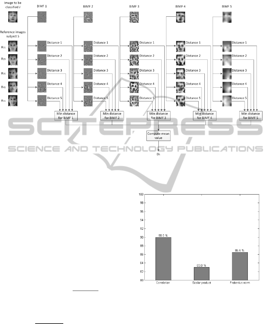
Figure 2: Scheme of the proposed image processing procedure for one image I to be classified. New Image I is compared
with the images reference R
is
of each subject. Distance between the same numbers of BIMF is computed and then the minim
distance is kept representing each BIMF. Minim distances are then averaged. Final value D
s
present the distance between
the new image and the subject. Distance is computed with all the subjects.
Figure 2 presents an application example for
explaining steps (iii) and (iv).
Hence, concerning to distances computed in
point (iii) three different measures are used in order
to explore and compare different configurations.
These measures are correlation, the matrix scalar
product and Frobenius norm. Considering two
matrixes and the computation of each distance
is done as follows:
1. Correlation coefficient between matrices
and.
2. Matrix scalar product, also known as the
normalized Frobenius inner product:
,
:
‖
‖
‖
‖
(11)
where : is the the Frobenius inner product of
the matrices and , defined as :
trace
, and
‖
‖
is the Frobenius norm defined
as
‖
‖
trace
, where
denotes the
transpose of a matrix.
3. Frobenius norm of the difference:
,
‖
‖
(12)
Figure 3: Obtained classification rates (%) for the three
different distances when the class association is based on
the minimum distance with each subject. Exact
experimental values are presented at the top of each bar.
3 RESULTS
This section presents the results after applying the
image processing to the data base and using the
described three different distances measures.
FaceRecognitionbyFastandStableBi-dimensionalEmpiricalModeDecomposition
389
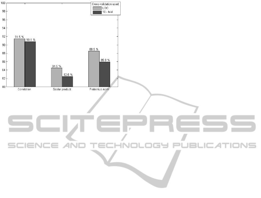
Figure 4: Obtained classification rates (%) for the three
different distances when LDA classification is used for the
class association. Exact experimental values are presented
at the top of each bar.
Figure 3 summarizes the obtained classification
results only based on the criterion of the minimum
distance. 90.0% of accuracy is obtained with
correlation, 83.0% is obtained when the used
measure is the scalar product, and 86.5% is obtained
with the Frobenius norm.
Figure 4 summarizes the obtained classification
results using LDA in the classification step. Results
obtained using LOOCV and 10-fold cross-validation
are presented. Interestingly, the use of LDA and
LOO cross-validation presents some small
improvement in the results. Classification rates (CR)
obtained using LOO cross-validation are 91.5%,
84.5% and 88.5% for correlation, scalar product and
Frobenius norm respectively. These results are
higher than results presented in Figure 3. However,
when the 10-fold cross-validation is applied, only
Correlation (which already presented the best result)
presents better CR than those obtained when the
class association is done only with the criterion of
the minimum distance. Results obtained for scalar
product and Frobenius norm present a decrease in
comparison with results showed in Figure 3.
These experiments show that results obtained
without any classifier are improved when LDA with
LOO cross-validation is used. However, the
variation is very small in these first experiments and
we will try to increase it in future research.
4 CONCLUSION AND
DISCUSSION
This study explores the use of FSBEMD for face
recognition. Distance measures are computed
between BIMFs obtained from reference images and
the image to classify. Then, class is assigned based
on the minimum distance between references and the
images of example, and also using a LDA classifier.
Obtained results do not overcome existing results
in the literature. Results presented in (Travieso et al.
2008) and in (Gallego-Jutglà et al. 2013) achieve a
98% of performance in the classification, which is
better than results presented in this work. However,
in the present work a more simple approach is used.
Results obtained in (Travieso et al. 2008) use a
DCT or DWT (Biorthonal 4.4 family)
parameterization, which is combined with a support
vector machine classifier. Here, the new FSBEMD
technique is used to decompose each image of the
data set and the vector of distance measures is used
alone or is given to a classifier (LDA or ANN). In
this case, the proposed system does not use any kind
of transformation (DCT, DWT or others).
On the other hand, results presented in (Gallego-
Jutglà et al. 2013) also present a CR of 98.25%. In
this work no transformation such as DCT, DWT or
others was applied. Methodology used in (Gallego-
Jutglà et al. 2013) was based on mEMD to compute
the joint decomposition of two images. Best result
obtained was found by classifying obtained
distances with an ANN. 98.25% of CR was achieved
when all measures were combined as input features
for the ANN, which may lead to overfitting.
However, when each measure was used alone, the
best result obtained was 97.25%. Another
shortcoming of the work presented in (Gallego-
Jutglà et al. 2013) is that if an implementation would
be done in a real system the mEMD of the image to
classify and all the existing images of the data base
would have to be computed. This procedure is time
consuming and therefore if the data base is big could
not be implemented in real time. Methods defined in
this work, however, compute the FSBEMD of an
image which is time consuming, but this
decomposition is only computed once.
Results presented here explore the two
dimensional information contained in the image.
Even though more information is used, results do not
overcome previous results that used only one
dimension. One possible shortcoming of the
presented methodology is that some information
may be lost in the average done to obtain the
distance value D
s
. Moreover, all extracted FSIMF
are used whereas some of them may not add any
new information but noise. This will be further
analysed in future work.
On the other hand, in this study the original size
BIOSIGNALS2015-InternationalConferenceonBio-inspiredSystemsandSignalProcessing
390

of the images have been used for the decomposition,
another further analysis may explore the
performance of the method by changing (reducing)
the size of the image, in order to decrease the
computational load of FSBEMD algorithm without
losing accuracy in the results.
The success of the proposed method is promising
and will encourage us to continue investigating the
use FSBEMD for image processing. In any case, the
method also needs to be tested with other databases
in order to ensure its general performance. In this
case the method has been tested in a database
containing face of subjects, but it could also be used
with images containing objects or biomedical
images.
ACKNOWLEDGEMENTS
This work has been partially supported by the
DAAD, Acciones Conjuntas Hispano – Alemanas
(2014), by the University of Vic – Central
University of Catalonia under the grant R0947, and
under a predoctoral grant from the University of Vic
– Central University of Catalonia to Mr. Esteve
Gallego-Jutglà, ("Amb el suport de l'ajut predoctoral
de la Universitat de Vic");
REFERENCES
Duda, R. O., Hart, P. E. & Stork, D.G., 1995. Pattern
Classification and Scene Analysis 2nd ed.
Fukunaga, K., 1990. Introduction to statistical pattern
recognition, Academic press.
Gallego-Jutglà, E. et al., 2013. Empirical mode
decomposition-based face recognition system. In
BIOSIGNALS 2013 - Proceedings of the International
Conference on Bio-Inspired Systems and Signal
Processing. pp. 445–450.
Iancu, C., Corcoran, P. & Costache, G., 2007. A Review
of Face Recognition Techniques for In-Camera
Applications. In 2007 International Symposium on
Signals, Circuits and Systems. IEEE, pp. 1–4.
Phillips, P. J. et al., 2011. An introduction to the good, the
bad, & the ugly face recognition challenge problem. In
Face and Gesture 2011. IEEE, pp. 346–353.
Sandwell, D. T., 1987. Biharmonic spline interpolation of
Geos-3 and Seasat altimeter data. Geophysical
Research Letters, 14(2), pp.139–142.
Travieso, C. M. et al., 2008. Reducción del vector de
características de reconocimiento facial. In XXII
Simposium de la Unión Científica Internacional de
Radio URSI’2008 Universidad Complutense de
Madrid.
Wagner, A. et al., 2012. Toward a practical face
recognition system: robust alignment and illumination
by sparse representation. IEEE transactions on pattern
analysis and machine intelligence, 34(2), pp.372–86.
Wessel, P. & Bercovici, D., 1998. Interpolation with
Splines in Tension: A Green’s Function Approach.
Mathematical Geology, 30(1).
Woodward, J.D., Orlans, N.M. & Higgins, P.T., 2002.
Biometrics: Identity Assurance in the Information Age,
McGrau-Hill.
Xiao, Q., 2007. Technology review - Biometrics-
Technology, Application, Challenge, and
Computational Intelligence Solutions. IEEE
Computational Intelligence Magazine, 2(2), pp.5–25.
FaceRecognitionbyFastandStableBi-dimensionalEmpiricalModeDecomposition
391
