Does Inverse Lighting Work Well under Unknown Response Function?

Shuya Ohta and Takahiro Okabe

Department of Artiﬁcial Intelligence, Kyushu Institute of Technology, Iizuka, Japan

Keywords:

Single-image Understanding, Inverse Lighting, Response Function, Lambertian Model.

Abstract:

Inverse lighting is a technique for recovering the lighting environment of a scene from a single image of an

object. Conventionally, inverse lighting assumes that a pixel value is proportional to radiance value, i.e. the

response function of a camera is linear. Unfortunately, however, consumer cameras usually have unknown and

nonlinear response functions, and therefore conventional inverse lighting does not work well for images taken

by those cameras. In this study, we propose a method for simultaneously recovering the lighting environment

of a scene and the response function of a camera from a single image. Through a number of experiments using

synthetic images, we demonstrate that the performance of our proposed method depends on the lighting dis-

tribution, response function, and surface albedo, and address under what conditions the simultaneous recovery

of the lighting environment and response function works well.

1 INTRODUCTION

Humans seem to extract rich information about an ob-

ject of interest even from a single image of the object.

Since the dawn of computer vision, understanding a

single image is one of the most important and chal-

lenging research tasks.

The appearance of an object depends on the shape

and reﬂectance of the object as well as the lighting

environment of a scene. From the viewpoint of physi-

cal image understanding, this means that the problem

of single-image understanding results in recovering

those three descriptions of a scene from a single im-

age. Unfortunately, however, such a problem is terri-

bly underconstrained;we havemultiple unknownsbut

only a single constraint per pixel. Therefore, conven-

tional techniques such as shape from shading (Horn,

1986) assume that two out of the three descriptions

are known and then recover the remaining one.

One direction of generalization of single-image

understanding is to recover two or three descriptions

from a single image. For example, Romeiro and Zick-

ler (Romeiro and Zickler, 2010) propose a method for

simultaneously recovering the reﬂectance of an object

and the lighting environment of a scene from a sin-

gle image of the object with known shape (sphere).

Barron and Malik (Barron and Malik, 2012) propose

a method for simultaneously recovering the shape,

albedo, and lighting environment from a single im-

age. Those methods exploit the priors, i.e. the statisti-

cal models of those descriptions, and search the most

likely explanation of a single image.

In this study, we focus on single-image under-

standing under unknown camera properties, that is

another direction of generalization. Existing meth-

ods for single-image understanding assume that a sin-

gle image is taken by an ideal camera and ignore the

effects of in-camera processing. They represent the

pixel values of the image as a function with respect

to the descriptions of a scene, i.e. shape, reﬂectance,

and lighting environment, and then recover some of

those descriptions from a single image. On the other

hand, we assume that a single image is taken by a

consumer camera and take in-camera processing in

particular tone mapping into consideration. We rep-

resent the pixel values of the image as a function with

respect to both the scene descriptions and the proper-

ties of a camera and camera setting, and then address

the recovery of scene descriptions from a single im-

age under unknown camera properties.

Inverse lighting (Marschner and Greenberg, 1997)

is a technique for recovering the lighting environment

of a scene from a single image under the assumptions

that the shape and reﬂectance (or basis images) of the

scene are known. Comparing with active techniques

using devices such as a spherical mirror (Debevec,

1998) and a camera with a ﬁsh-eye lens (Sato et al.,

1999) placed in a scene of interest, inverse lighting

is a passive technique and therefore could recover the

lighting environment from a given image taken even

in the past, although it is applicable to scenes with

relatively simple shape and reﬂectance.

Conventionally, inverse lighting assumes that a

pixel value is proportional to a radiance value at the

652

Ohta S. and Okabe T..

Does Inverse Lighting Work Well under Unknown Response Function?.

DOI: 10.5220/0005344406520657

In Proceedings of the 10th International Conference on Computer Vision Theory and Applications (VISAPP-2015), pages 652-657

ISBN: 978-989-758-089-5

 2015 SCITEPRESS (Science and Technology Publications, Lda.)

corresponding point in a scene. The relationship be-

tween radiance values and pixel values is described

by a radiometric response function, and the above as-

sumption means that the response function of a cam-

era is linear. Unfortunately, however, consumer cam-

eras usually have nonlinear response functions in or-

der to improve perceived image quality via tone map-

ping (Grossberg and Nayar, 2003). Therefore, con-

ventional inverse lighting requires a machine-vision

camera with a linear response function or radiometric

calibration of a response function in advance.

Accordingly, we propose a method for recover-

ing the lighting environment of a scene from a single

image taken by a camera with an unknown and non-

linear response function. Our proposed method also

assumes that the shape and reﬂectance of an object

are known, and then simultaneously estimates both

the lighting environment of a scene and the response

function of a camera from a single image. Speciﬁ-

cally, our method represents a lighting distribution as

a linear combination of the basis functions for light-

ing and also represents a response function as a linear

combination of the basis functions for response, and

then estimates those coefﬁcients from a single image.

We conduct a number of experiments using synthetic

images, and investigate the stability of our method.

We demonstrate that the performance of our method

depends on the lighting environment, response func-

tion, and surface albedo, and show experimentally un-

der what conditions the simultaneous recovery of the

lighting environment and response function from a

single image works well.

The main contribution of this study is twofold;

(i) the novel method for simultaneously recovering

the lighting environment of a scene and the response

function of a camera from a single image, and (ii) em-

pirical insights as to under what conditions inverse

lighting from a single image with an unknown re-

sponse function works well.

2 INVERSE LIGHTING

In this section, we explain the framework of in-

verse lighting on the basis of the original work by

Marschner and Greenberg (Marschner and Green-

berg, 1997). Inverse lighting assumes that the shape

and reﬂectance of an object are known, and then re-

covers the lighting environment of a scene from a sin-

gle image of the object. We assume that the object is

illuminated by a set of directional light sources, and

describe the intensity of the incident light from the di-

rection (θ, φ) to the object as L(θ, φ). Here, θ and φ

are the zenith and azimuth angles in the spherical co-

ordinate system centered at the object. Hereafter, we

call L(θ, φ) a lighting distribution.

Speciﬁcally, we represent a lighting distribution

L(θ, φ) by a linear combination of basis functions as

L(θ, φ) =

∑

n=1

(θ, φ), (1)

where α

and L

(θ, φ) (n = 1, 2, 3, ..., N) are the coef-

ﬁcients and basis functions for lighting. Then, based

on the assumption of known shape and reﬂectance,

we synthesize the basis images, i.e. the images of

the object when the lighting distributions are equal to

the basis functions for lighting L

(θ, φ). We denote

the p-th (p = 1, 2, 3, ..., P) pixel value of the n-th ba-

sis image by R

). According to the superposition

principle, the p-th pixel value of an input single image

(p = 1, 2, 3, ..., P) is described as

∑

n=1

). (2)

This means that we obtain a single constraint on the

coefﬁcients of lighting per pixel.

Rewriting the above constraints in a matrix form,

we obtain



















. . . R

) . . .



















,(3)

I = Rα. (4)

Since the P × N matrix R is known and the number

of pixels (constraints) P is larger than the number of

basis functions (unknowns) N in general, we can es-

timate the coefﬁcients of lighting α by solving the

above set of linear equations. Speciﬁcally, the coefﬁ-

cients are computed by using the pseudo inverse ma-

trix R

α = R

I = (R

⊤

−1

⊤

I, (5)

if R is full rank, i.e. the rank of R is equal to N.

This solution is equivalent to that of the least-square

method;

α = argmin

ˆα

∑

p=1

−

∑

n=1

)

. (6)

Once the coefﬁcients of lighting α are computed,

we can obtain the lighting distribution by substituting

them into eq.(1).

3 PROPOSED METHOD

In this section, we propose a method for simultane-

ously recovering both the lighting environment of a

DoesInverseLightingWorkWellunderUnknownResponseFunction?

653

scene and the response function of a camera from a

single image taken under an unknown and nonlinear

response function.

3.1 Representation of Lighting

Distribution

Our proposed method assumes that the shape of an

object is convex and the reﬂectance obeys the Lam-

bertian model, and then recovers the lighting dis-

tribution of a scene on the basis of the diffuse re-

ﬂection components observed on the object surface.

It is known that the image of a convex Lambertian

object under an arbitrary lighting distribution is ap-

proximately represented by a linear combination of

9 basis images when low-order spherical harmonics

(θ, φ) (l = 0, 1, 2; m = −l, −l + 1, ..., l − 1, l) are

used as the basis functions for lighting (Ramamoorthi

and Hanrahan, 2001). For the sake of simplicity, we

denote the spherical harmonics Y

(θ, φ) by Y

(θ, φ),

where n = (l + 1)

− l + m.

Substituting the spherical harmonics into eq.(1), a

lighting distribution L(θ, φ) is represented as

L(θ, φ) =

∑

n=1

(θ, φ). (7)

In a similar manner to eq.(2), the p-th pixel value of

the n-th basis image is represented as

∑

n=1

). (8)

Note that the pixel value I

is equivalent to the radi-

ance value when the response function of a camera is

linear.

The reason why the image of a convex Lamber-

tian object under an arbitrary lighting distribution is

approximated by using low-order spherical harmon-

ics is that high-frequency components of a lighting

distribution have no/little contribution to pixel val-

ues. In an opposite manner, we cannot recover the

high-frequency components of a lighting distribu-

tion from pixel values (Ramamoorthi and Hanrahan,

2001). This is the limitation of inverse lighting from

diffuse reﬂection components.

3.2 Representation of Response

Function

The radiance values of a scene are converted to pixel

values via in-camera processing such as demosaicing,

white balancing, and tone mapping. In this study, we

focus on tone mapping because it is widely used in

consumer cameras in order to improve perceived im-

age quality and the pixel values converted by tone

mapping are signiﬁcantly different from the radiance

values as shown in Figure 1 (a) and (b). As men-

tioned in Section 1, the relationship between radiance

values and pixel values is described by a radiometric

response function. In general, the response function

depends on cameras and camera settings.

Let us denote a response function by f , and as-

sume that a radiance value I is converted to a pixel

value I

′

by using the response function as I

′

= f(I).

Since the response function is monotonically increas-

ing, there exists the inverse of f, i.e. an inverse re-

sponse function g. The inverse response function con-

verts a pixel value I

′

to a radiance value I as I = g(I

′

and therefore has 255 degrees of freedom for 8-bit

images. Such a high degree of freedom makes the si-

multaneous recovery of a lighting distribution and a

response function from a single image intractable.

Accordingly, our proposed method uses an ef-

ﬁcient representation of response functions by con-

straining the space of response functions on the basis

of the statistical characteristics. Speciﬁcally, we make

use of the EMoR (Empirical Model of Response) pro-

posed by Greenberg and Nayar (Grossberg and Nayar,

2003). They apply PCA to the dataset of response

functions, and show that any inverse response func-

tion is approximately represented by a linear combi-

nation of basis functions as

I = g(I

′

) = g

′

) +

∑

m=1

′

). (9)

Here, β

and g

′

) are the coefﬁcients and basis

functions for response. Since the inverse response

function is also monotonically increasing, the coef-

ﬁcients has to satisfy

′

∑

m=1

′

) < g

′

+1)+

∑

m=1

′

+1),

(10)

where I

′

= 0, 1, 2, ..., 254 for 8-bit images.

3.3 Simultaneous Recovery

Substituting eq.(9) into the left-hand side of eq.(8),

we can derive

′

) =

∑

n=1

) −

∑

m=1

′

), (11)

i.e. a single constraint on the coefﬁcients of lighting

and response per pixel. We can rewrite the abovecon-

straints in a matrix form as

= (R|G)





, (12)

VISAPP2015-InternationalConferenceonComputerVisionTheoryandApplications

654

where g

= (g

′

), g

′

), ··· , g

′

))

⊤

and G is a

P× M matrix;

G =







··· −g

′

) ···







. (13)

If the P × (9+ M) matrix (R|G) is full rank, i.e. the

rank of (R|G) is (9+ M), we can compute both the co-

efﬁcients of the lighting distribution and those of the

response function by using its pseudo inverse matrix

in a similar manner to Section 2;





= (R|G)

. (14)

This solution is equivalent to that of the least-

square method;

{α, β} = argmin

ˆα,

∑

p=1

′

)−

∑

n=1

∑

m=1

′

)

.(15)

Since the response function is monotonically increas-

ing, we solve eq.(15) subject to eq.(10). We used the

MATLAB implementation of the trust-region reﬂec-

tive algorithm for optimization. In the experiments,

we set M = 5. Once the coefﬁcients of lighting α and

those of response β are computed, we can obtain the

lighting distribution and response function by substi-

tuting them into eq.(7) and eq.(9).

In order to make the simultaneous recovery of

lighting and response more stable, we can incorpo-

rate the priors of lighting distributions and response

functions into the optimization. For example, we can

add the smoothness term with respect to the response

function

255

∑

l=1

∂

g(I

′

)

∂I

′2



′

255

(16)

to eq.(15), where w is a parameter that balances the

likelihood term and the smoothness term. In our pre-

liminary experiments, we tested some simple priors

and found that we often need to ﬁne-tune the param-

eters of the priors according to input images. There-

fore, we do not use any priors in this study and investi-

gate the stability of the linear least-square problem in

eq.(15) with the linear constraints in eq.(10) instead.

4 EXPERIMENTS AND

DISCUSSION

In this section, we conduct a number of experiments

using synthetic images, and investigate the stability

100

200

300

400

500

600

0 50 100 150 200 250

Frequency

Pixel Value

0.2

0.4

0.6

0.8

0 0.2 0.4 0.6 0.8 1

Radiance Value

Pixel Value

(a) (b) (c)

(d) (e) (f)

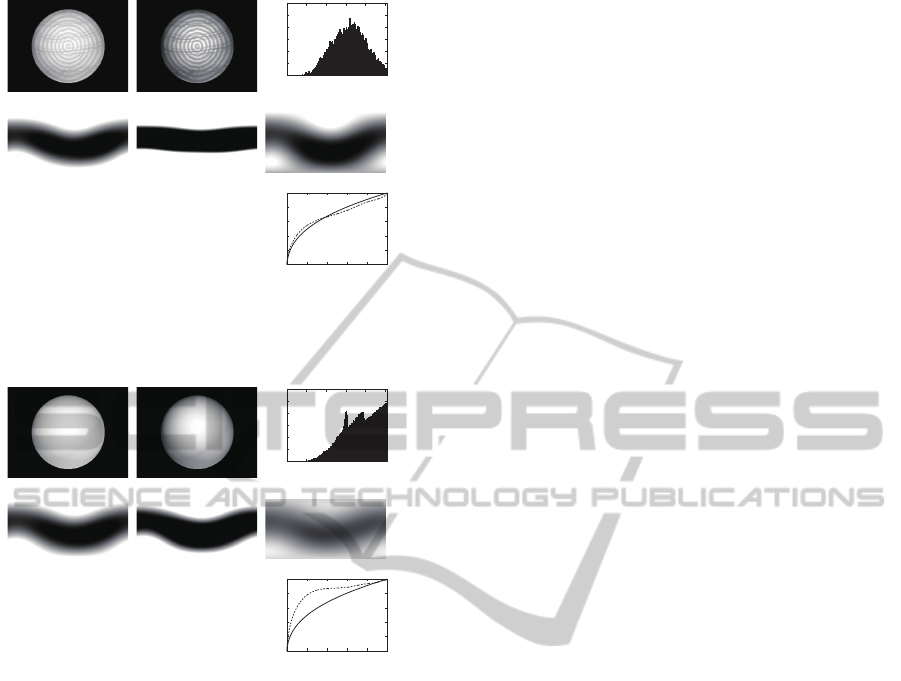
(g)

Figure 1: Recovered lighting distributions and response

function from a single image of an object under a single

directional light source.

Table 1: The RMS errors of the estimated response func-

tions.

Case

A B C D E

RMSE 0.09 0.10 0.54 0.04 0.13

of our proposed method. We can see from eq.(12) and

eq.(14) that the stability of our method is described by

the full rankness of the matrix (R|G) or the condition

number of the pseudo inverse matrix (R|G)

Each column of the sub-matrix R corresponds to

a basis image of an object illuminated by spherical-

harmonics lighting. It is known that the basis images

are orthogonal to each other if the surface normals

of the object distribute uniformly on a unit sphere

because spherical harmonics are orthonormal basis

functions on a unit sphere (Ramamoorthi and Han-

rahan, 2001). Intuitively, inverse lighting works well

for spherical objects but does not work for planar ob-

jects. In this study, we assume spherical objects and

therefore the sub-matrix R is full rank.

Each column of the sub-matrix G corresponds to

an eigenvector of response functions, and therefore

the columns are orthogonal to each other if the pixel

valuesin a single image distribute uniformly from 0 to

255. Intuitively, the simultaneous recovery of lighting

distribution and response function works well when

the histogram of the pixel values is uniform. Because

the pixel values in the image of a spherical object de-

pend on the lighting distribution of a scene, the re-

sponse function of a camera, and the surface albedo

of the object, we demonstrate how the performance

of our method changes depending on the lighting dis-

tribution, response function, and surface albedo.

Case A:

In Figure 1, we show images of a sphere under a

single directional light source with a linear response

function (a) and with a nonlinear response function

DoesInverseLightingWorkWellunderUnknownResponseFunction?

655

(a) (b) (c)

(d) (e) (f)

(g)

200

400

600

800

1000

1200

1400

1600

1800

2000

0 50 100 150 200 250

Frequency

Pixel Value

0.2

0.4

0.6

0.8

0 0.2 0.4 0.6 0.8 1

Radiance Value

Pixel Value

Figure 2: Results when only the lighting distribution is dif-

ferent from Figure 1.

(b). The histogram of the pixel values in the tone-

mapped image (b) is shown in (c). Figure 1 (d) shows

the lighting distribution estimated from the linear im-

age (a) by using the conventional method assuming a

linear response function (see Section 2). Here, the

lighting distribution L(θ, φ) is represented by a 2D

map whose vertical and horizontal axes correspond

to the zenith angle θ and azimuth angle φ respec-

tively. Figure 1 (e) and (f) show the lighting distri-

butions estimated from the tone-mapped image (b)

by using the conventional method and our proposed

method respectively. In Figure 1 (g), the solid and

dotted lines stand for the ground truth and estimated

response function by using our method.

We can see that the lighting distribution estimated

by using our proposed method (f) looks more sim-

ilar to (d) than that estimated by using the conven-

tional method (e). Since inverse lighting based on dif-

fuse reﬂection components cannot estimate the high-

frequency components of a lighting distribution as

mentioned in Subsection 3.1, (d) is considered to

be the best possible result. Therefore, those results

demonstrate that our method works better than the

conventional method for the tone-mapped image. In

addition, (g) demonstrates that the response function

estimated by using our method is similar to the ground

truth in some degree. The root-mean-square (RMS)

errors of the estimated response functions are shown

in Table 1.

Case B:

In Figure 2, we show the results when only the light-

ing distribution is different from Figure 1. Specif-

ically, a single directional light source and a uni-

form ambient light are assumed. Comparing the light-

ing distributions estimated by using the conventional

method (e) and our proposed method (f) with the best

possible result (d), we can see that our method out-

(a) (b) (c)

(d) (e) (f)

(g)

200

400

600

800

1000

1200

1400

1600

1800

2000

0 50 100 150 200 250

Frequency

Pixel Value

0.2

0.4

0.6

0.8

0 0.2 0.4 0.6 0.8 1

Radiance Value

Pixel Value

Figure 3: Results when only the response function is differ-

ent from Figure 1.

performs the conventional method. In addition, (g)

shows that the response function estimated by using

our method is similar to the ground truth in some de-

gree.

Those results demonstrate that the performance of

our method depends on lighting distributions. Al-

though the performance of our method is not perfect,

our method works well for both the case A and the

case B, and outperforms the conventional method.

Case C:

In Figure 3, we show the results when only the re-

sponse function is different from Figure 1. Compar-

ing (e) and (f) with (d), it is clear that our method

does not work well. In addition, (g) shows that the

response function estimated by using our method is

completely different from the ground truth.

Those results demonstrate that the performance of

our method depends also on response functions and

that our method does not work well for the case C.

The histogram of the pixel values in the tone-mapped

image (c) shows that the range of pixel values is sig-

niﬁcantly reduced due to the tone mapping. Compar-

ing Figure 1 (g) with Figure 3 (g), we can see that the

simultaneous recovery works well when the inverse

response function is convex upward, i.e. expands the

range of pixel values, but does not work well when it

is convex downward, i.e. shrinks the range of pixel

values.

Case D:

In Figure 4, we show the results when the image of

a textured sphere under four directional light sources

is used. Comparing (e) and (f) with (d), we can see

that our method works better than the conventional

method. In addition, (g) shows that our method can

estimate the response function accurately.

VISAPP2015-InternationalConferenceonComputerVisionTheoryandApplications

656

(a) (b) (c)

(d) (e) (f)

(g)

0.2

0.4

0.6

0.8

0 0.2 0.4 0.6 0.8 1

Radiance Value

Pixel Value

100

200

300

400

500

600

0 50 100 150 200 250

Frequency

Pixel Value

Figure 4: Recovered lighting distributions and response

function from a single image of a textured object under four

directional light sources.

(a) (b) (c)

(d) (e) (f)

(g)

100

200

300

400

500

600

0 50 100 150 200 250

Frequency

Pixel Value

0.2

0.4

0.6

0.8

0 0.2 0.4 0.6 0.8 1

Radiance Value

Pixel Value

Figure 5: Results when only the surface albedo is different

from Figure 4.

Case E:

In Figure 5, we show the results when only the sur-

face albedo is different from Figure 4. Comparing (e)

and (f) with (d), we can see that our method does not

necessarily work well. In addition, (g) shows that the

response function estimated by using our method de-

viates from the ground truth to some extent.

Those results demonstrate that the performance of

our method depends also on the surface albedo of an

object and that our method works better for textured

objects. The effects of texture can be explained as

follows. First, non-uniform albedo makes the distri-

bution of pixel values diverse. Second, more impor-

tantly, two pixels with similar surface normals but dif-

ferent reﬂectance values yield a strong constraint on

the response function. Since the irradiance values at

the pixels with similar surface normals are also simi-

lar to each other, the radiance values converted from

the pixel values at those pixels by using the inverse

response function should be proportional to their re-

ﬂectance values.

5 CONCLUSION AND FUTURE

WORK

In this study, we extended inverse lighting by tak-

ing an unknown and nonlinear response function of a

camera into consideration, and proposed a method for

simultaneously recovering the lighting environment

of a scene and the response function of a camera from

a single image of an object. Through a number of

experiments, we demonstrated that the performance

of our proposed method depends on the lighting dis-

tribution, response function, and surface albedo, and

addressed under what conditions the simultaneous re-

covery works well.

One of the future directions of this study is to in-

corporate sophisticated priors in order to make the si-

multaneous recovery more stable. Another direction

is to make use of other cues such as specular reﬂec-

tion components and cast shadows in order to recover

high-frequency components of a lighting distribution.

ACKNOWLEDGEMENTS

A part of this work was supported by JSPS KAK-

ENHI Grant No. 26540088.

REFERENCES

Barron, J. and Malik, J. (2012). Shape, albedo, and illumi-

nation from a single image of an unknown object. In

Proc. IEEE CVPR2012, pages 334–341.

Debevec, P. (1998). Rendering synthetic objects into real

scenes: bridging traditional and image-based graphics

with global illumination and high dynamic range pho-

tography. In Proc. ACM SIGGRAPH’98, pages 189–

198.

Grossberg, M. and Nayar, S. (2003). What is the space

of camera response functions? In Proc. IEEE

CVPR2003, pages 602–609.

Horn, B. (1986). Robot vision. MIT Press.

Marschner, S. and Greenberg, D. (1997). Inverse lighting

for photography. In Proc. IS&T/SID Fifth Color Imag-

ing Conference, pages 262–265.

Ramamoorthi, R. and Hanrahan, P. (2001). A signal-

processing framework for inverse rendering. In Proc.

ACM SIGGRAPH’01, pages 117–128.

Romeiro, F. and Zickler, T. (2010). Blind reﬂectometry. In

Proc. ECCV2010, pages 45–58.

Sato, I., Sato, Y., and Ikeuchi, K. (1999). Acquiring a radi-

ance distribution to superimpose virtual objects onto a

real scene. IEEE TVCG, 5(1):1–12.

DoesInverseLightingWorkWellunderUnknownResponseFunction?

657