Computing Attributes of Software Architectures

A Static Method and Its Validation

Imen Derbel

, Lamia Labed Jilani

and Ali Mili

Institut Superieur de Gestion, Bardo, Tunisia

New Jersey Institute of Technology, Newark, NJ, 07102-1982, U.S.A.

Keywords:

Software Architecture, Architecture Description Language, Analysis, Quality Attributes, Acme, Response

Time, Throughput, Reliability.

Abstract:

During the last two past decades, software architecture has been a rising subject of software engineering.

Since, researchers and practitioners have recognized that analyzing the architecture of a software system is

an important part of the software development process. Architectural evaluation not only reduces software

development efforts and costs but it also enhances the quality of the software by verifying the addressability

of quality requirements and identifying potential risks. To this aim, several approaches have been recently

proposed to analyze system non-functional attributes from its software architecture speciﬁcation.

In this paper, we propose an ADL based formal method for representing and reasoning about system non-

functional attributes at the architectural level. We are especially interested in analyzing performance and

reliability quality attributes. We also propose to analyze the sensitivity of the system by identifying compo-

nents that have the greatest impact on the system quality. The automation of our model was followed by a

series of experiments that allowed us to validate our inductive reasoning to prove the capabilities of our model

to represent and analyze software architectures.

1 INTRODUCTION

Software Architecture is a rising subject of software

engineering that helps people to oversee a system in

high level. It is deﬁned as the system structure(s),

which comprise software elements, the externally vis-

ible properties of those elements, and the relation-

ships between them (Bass et al., 1998).

The architecture of a software product is tradition-

ally modeled from the requirements speciﬁcation, ac-

cording to the needs expressed by one or more clients.

The speciﬁcation expresses customer needs in terms

of service functions, constraints, quality, etc. From

the speciﬁcations, the designers propose one or more

solutions that meet the customer needs. At this stage,

we must ensure that these proposed alternatives meet

all requirements speciﬁcation to pass the later stages

of the life cycle (eg. implementation, integration,

etc.). It is therefore recommended to develop methods

and tools to analyze non-functional properties of soft-

ware architectures to provide designers with a sup-

port in their activities. Analysis of the product early

in the software life cycle, helps not only to discover

the problems of the architecture but also to make de-

cisions reﬁnements of software products upstream.

This reduces software development efforts and costs,

and enhances the quality of the software by verifying

the addressability of quality requirements and identi-

fying potential risks.

In this context, several approaches have been pro-

posed in order to analyze systems quality attributes

at the architectural level. However, despite capacities

of architecture description languages (ADLs) in for-

mal description of software architectures, there is a

notable lack of support for non-functional attributes

in existing ADLs. Acme, Aesop, Weaves and others

allow the speciﬁcation of arbitrary component proper-

ties, but none of them interprets such properties nor do

they make direct use of them (Medvidovic and Taylor,

2000).

In this paper, we propose an ADL based formal

method for representing and reasoning about system

non-functional attributes at the architectural level. We

are interested in analyzing performance attributes (re-

sponse time and throughput) and reliability (failure

probability). We aim to compile an architectural de-

scription and obtain a set of equations that charac-

terize non-functional attributes of software architec-

Derbel I., Labed Jilani L. and Mili A..

Computing Attributes of Software Architectures - A Static Method and Its Validation.

DOI: 10.5220/0005347300550066

In Proceedings of the 10th International Conference on Evaluation of Novel Approaches to Software Engineering (ENASE-2015), pages 55-66

ISBN: 978-989-758-100-7

 2015 SCITEPRESS (Science and Technology Publications, Lda.)

tures, using an inductive reasoning. These equations

are then solved using Mathematica (

Wolfram Re-

search) in order to obtain system properties as func-

tion of components and connectors properties. We

also propose to analyze the system performance sen-

sitivity and the system reliability sensitivity by iden-

tifying architectural components and connectors that

limit the system quality and that need an urgent at-

tention to be improved. In this paper, we report on

our experimentation of our approach on Aegis system

(Allen and Garlan, 1996). The goal here is to val-

idate the inductive reasoning and the model we have

proposed. First, we analyzed the non-functionalprop-

erties of Aegis using our ADL based approach. Then,

we simulate the performance of the Aegis system to

determine and calculate its response time, its through-

put and its reliability.

This paper is organized as follows. Section 2

presents the background and the related work. Section

3 introducesACME+ ADL and presents the main syn-

tactic features that we have added to Acme. Section

4, describes the compiler that we propose for analyz-

ing ACME+ descriptions. Section 5, discusses per-

formance and reliability sensitivity analysis. Section

6, presents the generation of an automated tool for

the proposed analysis model. Section 7 outlines ex-

periments that we have conducted to validate our in-

ductive reasoning and analysis model. Section 8 con-

cludes this paper.

2 RELATED WORK

Several methods have been proposed for evaluating

software architectures quality attributes. These meth-

ods can be categorized as either being informal meth-

ods (including experience-based, simulation-based,

scenario-based approaches) or being formal ones (in-

cluding mathematical modeling based approaches)

(Bosch, 1999).

Some approaches are interested to the qualitative

analysis (Giannakopoulou et al., 1999), (wr2, 2005),

they verify structural and behavioral properties of the

software product such properties are: vivacity, live-

ness, coherence, blocking free, etc. While some other

approaches focus on quantitative analysis, they calcu-

late the values of software product measurable prop-

erties such as performance, reliability, availability,

maintainability, etc. Our approach falls into formal

analysis of quantitative quality attributes. In this con-

text, a number of mathematical modeling-based soft-

ware architecture evaluation methods have been de-

veloped. These methods model software architectures

using well-known formalisms and models. Then,

these models are used to estimate operational qual-

ity attributes. However, each approach analyzes only

one attribute, either reliability or performance.

In the following, we ﬁrst discuss different ap-

proaches for assessing performance of a software ar-

chitecture. Then, we discuss the approaches for pre-

dicting reliability at the architectural level.

Several studies address the performance assess-

ment from a software architecture description. Each

approach is based on a certain type of performance

model and speciﬁcation language. The latter includes

speciﬁcation formalisms such as ADL descriptions,

Chemical abstract machine, and UML based speciﬁ-

cation. Performance models include Stochastic Pro-

cess Algebras, queueing networks (QN) and their ex-

tensions called Extended Queueing Networks (EQN)

and Layered Queueing Networks (LQN), etc.

QN is one of the best known performance models.

Aquilani et al., in (Aquilani et al., 2001), proposed

the derivation of QN models from Labeled Transi-

tion Systems (LTS) describing the dynamic behavior

of SAs. Spitznagel and Garlan, in (Spitznagel and

Garlan, 1998), proposed the transformation of Acme

descriptions to QN models using ”distributed message

passing” style deﬁned in Aesop ADL. However, they

propose only performance analysis of client/server

systems. Bernardo et al. in (Balsamo et al., 2002) pro-

posed Æmilia, an architectural description language

based on stochastic Process Algebra that allows to

solve performance indices using Timed Markov Mod-

els.

Several studies address the reliability assessment

from a software architecture description. Goseva-

Popstojanova and Trivedi (Goseva-Popstojanova and

Trivedi, 2001) classify these approaches into three

categories: state-based, path-based and additive. We

discuss the path-based and the state-based approaches

while ignoring the additive approach as it is not di-

rectly related to software architecture.

Path-based approaches (Shooman, 1976), (Krish-

namurthy and Mathur, 1997) assess the reliability of

the system according to the possible execution paths

of the program, which can be obtained experimen-

tally, by testing or algorithmically. In other words,

the reliability of each path is obtained as a product

of the reliabilities of the components along that path.

Then, the system reliability is calculated by averag-

ing the reliability of all the paths. One of the major

problems with the path-based approaches is that they

provide only an approximate estimate of application

reliability (Franco et al., 2012).

State-based approaches (Cheung, 1980), (Franco

et al., 2012), (Gokhale, 2007) assume that the transi-

tions between states havea Markov property, meaning

ENASE2015-10thInternationalConferenceonEvaluationofNovelSoftwareApproachestoSoftwareEngineering

that at any time the future behaviour of components

or transitions between them is conditionally indepen-

dent of the past behaviour. These models consider

software architectures as a discrete Markov chain

(DTMC) or a continuous time Markov chain (CTMC)

or a semi-Markovprocess (SMP) which are solved us-

ing probabilistic model checking tools such as Prism

(Kwiatkowska et al., 2009). However, Markov mod-

els face a common problem, the combinatorial growth

of the statespace. This occurs when the model has a

large number of states and a great number of tran-

sitions between those states exceeding the memory

available.

3 ACME+: AN ARCHITECTURAL

DESCRIPTION LANGAGE

In order to support the automated derivation of syn-

thesized attributes from the attributes of building

components and connectors, an ADL needs to have

two important features: constructs to represent rele-

vant attributes and constructs to represent functional

dependencies between components and connectors.

These two constructs are needed to reason about how

attributes are synthesized throughout the architecture.

For the purposes of our study, we deﬁne an ADL

called ACME+ as an extension of Acme ADL.

Acme was selected for extension because it is an

interchange language offering beneﬁts from the com-

plementary capabilities of ADLs. Also, it is supported

by AcmeStudio tool which enables users to edit archi-

tectures via a graphical user interface. In addition, it

offers a complete ontology to describe software ar-

chitectures, distinguishing between various architec-

tural elements: components, connectors, and conﬁg-

uration. The construct of

functional dependency

arises from the observation that the topological infor-

mation represented by Acme is not sufﬁcient to de-

rive synthesis rules for the various attributes, and con-

sists primarily in deﬁning relationships between the

various ports of an Acme component and the various

roles of an Acme connector. To ﬁx our ideas, we fo-

cus on functional dependencies within a component,

which represent the relationships between the ports

of a component. At a minimum, the

functional

dependency

must specify which ports are used for

input

and which ports are used for

output

. In ad-

dition, for input ports, we must specify whether the

component may proceed with data from any one of

the ports (

AllOf

) or the component needs data from

all ports before it proceeds (

AnyOf

); also, there are

cases where we may need a majority of input ports to

proceed (

MostOf

), such as in a modular redundancy

scheme (for example, we have three input ports pro-

viding duplicate information, and we proceed as soon

as two out of the three produce the same input data).

As an example, let a component C has, say ﬁve

ports, P1, P2, P3, P4, P5 and we wish to record that

P1, P2, P3 are the input ports, then, depending on

which conﬁguration we want to represent, we write:

input(AllOf(P1,P2,P3)),

input(AnyOf(P1,P2,P3)),

input(MostOf(P1,P2,P3)).

In the latter two cases, we must also specify

whether the input ports must deliver their inputs

synchronously

asynchronously

. Hence we

could say, for example:

input(AllOf(asynch(P1,P2,P3)),

input(MostOf(synchro(P1,P2,P3)).

As for output ports, in case we have more than one

for a given component, we may represent two as-

pects: the degree of overlap between the data on

the various ports (

duplicate

exclusive

overlap

and the synchronization between the output ports

(

simultaneous

asavailable

). Pursuing the exam-

ple discussed above, if P4 and P5 are output ports,

then we can write, depending on the situation:

output(overlap(asavailable(P4,P5)),

output(exclusive(simultaneous(P4,P5)),

output(exclusive(asavailable(P4,P5)).

In ACME+, a functional dependency is written at the

end of a component description, after the declaration

of all the ports, or at the end of a connector descrip-

tion, after the declaration of all the roles. A declara-

tion of a

functional dependency

has the following

ﬁelds:

• a name, to identify the dependency,

• a declaration of the input relation (how input ports

are coordinated),

• a declaration of the output relation (how output

ports are coordinated),

• a declaration of relevant properties (e.g. process-

ing time for components, transmission time for

connectors, etc).

As an example, we may write:

FunDep { Name_of_functional_dependency

input (MostOf(synchro(P1,P2,P3))),

output(exclusive(asavailable(P4,P5))),

properties(processingTime=0.02,

throughput = 45,failureProbability = 0.03)}

ComputingAttributesofSoftwareArchitectures-AStaticMethodandItsValidation

4 A COMPILER FOR ACME+

ARCHITECTURE

We have developed a compiler for ACME+; while

programming language compilers map source code

onto executable code, our compiler maps ACME+

source code onto a set of Mathematica equations that

characterize the non functional attributes of the ar-

chitecture of interest. To this effect, we assume that:

all ports of components are labeled for

input

or for

output

(

input

ports feed data or control information

to the component, and

output

ports receive data or

control information from the component); all roles of

connectors are labeled as

origin

or as

destination

(connectors carry data or control information from

their

origin

roles to their

destination

roles); there

is a single component without input port and with a

single output port, called the

source

; there is a single

componentwithout output port and with a single input

port, called the

sink

; we assume that the

source

and

sink

components are both dummy components, that

are used solely for the purposes of our model (if the

architecture happens to have a real component with-

out input port and with a single output port, we pro-

vide it an input port and we attach a dummy source

component and a dummy connector upstream of it;

likewise for the sink component). We deﬁne an at-

tribute grammar on such architectures, as follows:

• Each port of each component has an attribute for

each property of interest (response time, through-

put, failure probability); hence each port has

three attributes, labeled RT (response time), TP

(throughput), FP (failure probability).

• Likewise, each role of each connector has an at-

tribute for each property of interest, labeled the

same way.

• The output port of the source component has triv-

ial values for all the attributes, namely:

source.inpPort.RT = 0,

source.inpPort.TP = infinity,

source.inpPort.FP = 0.

• The system inherits the attributes associated to the

input port of the sink component, namely:

System.ResponseTime = sink.outPort.RT,

System.Throughput = sink.outPort.TP,

System.FailureProbability = sink.outPort.FP.

The question that we must address now is, of course,

how do we compute the attributes of the sink from the

properties of components and connectors. We do so

by propagating attributes from the

source

to the

sink

in a stepwise manner, by considering the following

information:

• The functional dependency of each component, as

a relation between its input ports and output ports.

• The functional dependencyof each connector,as a

relation between its origin roles and its destination

roles.

• The relevant properties of each component. For

example, each component has a property called

Processing Time, that may come in handy when

we want to compute the value of the RT (response

time) attribute of its output ports as a function of

the value of the RT attribute of its input ports.

• The relevant properties of each connector. For

example, each connector has a property called

Transmission Time, that may come in handy when

we want to compute the value of the RT (response

time) attribute of its destination roles as a function

of the value of the RT attribute of its origin roles.

• Whenever a port is attached to a role, the attribute

values are passed forward from the output port to

the source role. For each attachment of the form:

C.outPort to N.originRole.

We write:

C.outPort.RT = N.originRole.RT,

C.outPort.TP = N.originRole.TP,

C.outPort.FP = N.originRole.FP.

What remains to explain now is how the attributes

are propagated from input ports to output ports

within a component and from origin roles to des-

tination roles within a connector.

Let C designates a component, whose input ports

are called inPort

;...;inPort

and output ports are

called outPort

;...;outPort

. We suppose that these

input and output ports are related with a

functional

dependency

relation R expressed as follows:

Input(InSelection(InSynchronisation

(inPort1; ..; inPortn)));

Output(OutSelection(OutSynchronisation

(outPort1; ..; outPortk)));

Properties(procTime=0.7;thruPut=0.2;failProb=0.2)

)

We review in turn the three attributes of interest.

4.1 Response Time

For each output port outputP

expressed in the rela-

tion R, we write:

C.outPort

.RT = function(C.inPort1.RT;

...;C.inPort

.RT) +C.R. procTime.

(1)

where function depends on the construct

InSelection

, expressing the nature of the rela-

tion between input ports.

ENASE2015-10thInternationalConferenceonEvaluationofNovelSoftwareApproachestoSoftwareEngineering

If InSelection is AllOf, then function is the maxi-

mum, we write:

C.outPort

.RT = Max(C.inPort

.RT;...;C.inPort

.RT)

+C.R. procTime.

(2)

If InSelection is AnyOf, then function is the mini-

mum, we write:

C.outPort

.RT = Min(C.inPort

.RT;...;C.inPort

.RT)

+C.R. procTime.

(3)

If InSelection is MostOf, then function is the median,

we write:

C.outPort

.RT = Med(C.inPort

.RT;...;C.inPort

.RT)

+C.R. procTime.

(4)

4.2 Throughput

For each output port outPort

of the component C ex-

pressed in the relation R, we write an equation relating

the component’s throughput and inPort

.TP. This rule

depends on whether all of inputs are needed, or any

one of them. Consequently if InSelection is AllOf,

and since the slowest channel will impose its through-

put, keeping all others waiting, we write:

C.outPort

.TP = Min(C.R.thruPut;

(C.inPort

.TP+ ... +C.inPort

.TP)).

(5)

Alternatively, if InSelection is AnyOf, since the

fastest channel will impose its throughput, we write:

C.outPort

.TP = Max(Min[C.R.thruPut;C.inPort

.TP];

...;Min[C.R.thruPut;C.inPort

.TP]).

(6)

If InSelection is MostOf, then we write:

C.outPort

.TP = Min(C.R.thruPut;

(C.inPort

.TP+ ... +C.inPort

.TP) ÷ n).

(7)

4.3 Failure Probability

For each output port outPort

of the component C ex-

pressed in the relation R, we write an equation relating

component’s failure probability and failure probabil-

ities of its input ports. This rule depends on whether

all of inputs are needed, or any one of them. We ﬁrst

consider that inPort

, i = 0..n, provides complemen-

tary information (InSelection is AllOf). A compu-

tation initiated at C.outPort

will succeed if the com-

ponent C succeeds, and all the computations initiated

at the input ports of C succeed. Assuming statistical

independence, the probability of these simultaneous

events is the product of probabilities. Hence we write:

C.outPort

.FP = 1−

(1− C.inPort

.FP× ... ×C.inPort

.FP)

(1− C.R.FailProb).

(8)

Second we consider that inPort

provide interchange-

able information (InSelection is AnyOf). A compu-

tation initiated at C.outputP

will succeed if compo-

nentC succeeds, and one of the computations initiated

at input ports C.inPort

succeeds. Whence we write:

C.outPort

.FP = 1− (1−C.inPort

.FP) × ...

×(1− C.inPort

.FP)(1−C.R.FailProb).

(9)

If InSelection is MostOf,then we write:

C.outPort

.FP = 1− (1−C.R.FailProb)×

(1− (C.inPort

.FP+ ... +C.inPort

.FP) ÷ n).

The ACME+ compiler generates all the equations that

we have discussed in this section in Mathematica for-

mat, to enable us to reason about the non functional

attributes of the overall system, as a function of the

relevant properties of its components and connectors,

its functional dependencies, and its topology.

5 SENSITIVITY ANALYSIS

Sensitivity analysis informs architects about what are

the architectural constituents that need an urgent at-

tention to be improved. So they can improve a soft-

ware architecture, test and validate it based on its

components and connectors properties, architectural

style, etc. Therefore, we developed a performance

and reliability sensitivity analysis able to help archi-

tects identify architectural components that require

changes.

5.1 Performance Sensitivity Analysis

Performance sensitivity analysis consists in identify-

ing component bottleneck that limits the system per-

formance. Hence, we have used queueing networks

laws. We present below the most important two laws

(equations 10 and 11) that we have used. A more

detailed explanation can be found in (Denning and

Buzen, 1978). Let D

be the total service demand on

the constituent i (component or connector). D

is de-

ﬁned by :

× S

(10)

where X

and S

are respectively the processing time

and the throughput of constituent i. The system

ComputingAttributesofSoftwareArchitectures-AStaticMethodandItsValidation

throughput X veriﬁes the following inequality:

X ≤

(11)

Therefore, the constituent with largest D

limits the

system throughput and is the bottleneck. Since in our

model, each constituentC is described by one or more

functional dependency

relations and each relation

R is characterized by a processing time, we propose

to calculate service demand D

of constituent C rel-

ative to each relation R

. D

is deﬁned by:

(C.R

.thruPut×C.R

. procTime)

System.Throughput

(12)

The constituent having the largest value of D

, is the

bottleneck of the system.

5.2 Reliability Sensitivity Analysis

Reliability sensitivity analysis consists in identifying

component bottleneck that limits the system reliabil-

ity. Let’s recall that the equations generated by our

compiler will be resolved by Mathematica numeri-

cally and symbolically. The symbolic resolution is to

keep components and connectors properties unspeci-

ﬁed and use Mathematica to produce a system prop-

erty expression based on components and connectors

properties. This form of resolution helps in analyz-

ing the sensitivity with respect to reliability. Note

that our model allows the analysis of system fail-

ure probability according to components and connec-

tors failure probabilities. To determine which compo-

nent/connector that most affects system reliability, we

calculate the derivative of the system failure probabil-

ity with respect to its components/connectors failure

probabilities. The derivative of the formula is deﬁned

by the equation 13:

∂System.FailProb

∂C

.FailProb

;i = 1, 2, ..., n (13)

where C

is the component/connector i. The compo-

nent/connector having the highest value of the deriva-

tive is the reliability bottleneck.

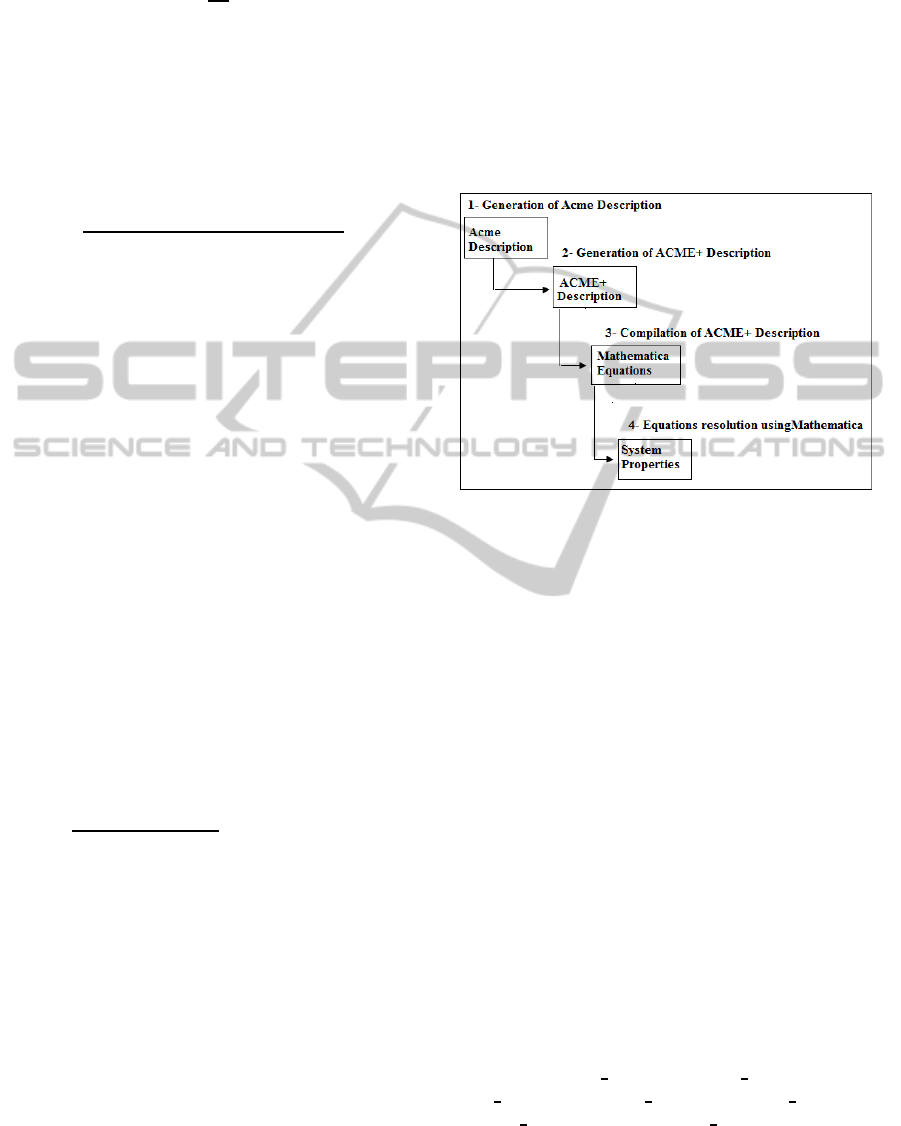
6 AN AUTOMATED TOOL FOR

ARCHITECTURE ANALYSIS

We have developed an automated tool that analyzes

architectures according to the pattern discussed in this

paper. This tool uses a compiler to map the architec-

ture written in ACME+ onto Mathematica equations,

then it invokes Mathematica to analyze and solve the

resulting system of equations. The analysis process

is illustrated by ﬁgure 1. It can be observed that

our analysis tool takes as input a ﬁle containing a

given system architecture description written in our

enriched ACME+ ADL. The compiler then translates

this ﬁle into mathematical equations that characterize

the system’s non-functional attributes. Then, the tool

invokes Mathematica to compute actual values of the

system’s attributes or to highlight functional depen-

dencies between the attributes of the system and the

attributes of the system’s components and connectors.

Figure 1: Analysis process workﬂow.

7 EXPERIMENTS

Our work consists in analyzing quantitative non-

functional requirements that can inductively be de-

rived such as response time, throughput, failure prob-

ability, etc. In order to validate our inductive ap-

proach, we propose to analyze the Aegis system

(Allen and Garlan, 1996) using our ACME+ based

method and verify the obtained results by simulating

the system architecture.

7.1 ACME+ Analysis of Aegis System

Aegis Weapons System (Allen and Garlan, 1996) is

designed to defend a battle group against air, sur-

face and subsurface threats. These weapons are

controlled through a large number of control con-

soles, which provide a wide variety of tactical de-

cision aids to the crew. Figure 2 depicts the ba-

sic architecture of Aegis represented in AcmeStudio

(Kompanek, 1998). The system consists of seven

components: Geo

Server, Doctrine Reasoning, Doc-

trine Authoring, Track Server, Doctrine Validation,

Display

Server and Experiment Control. To this con-

ﬁguration, we add, for the sake of illustration, two

dummy components Sink and Source and their asso-

ciated connectors.

ENASE2015-10thInternationalConferenceonEvaluationofNovelSoftwareApproachestoSoftwareEngineering

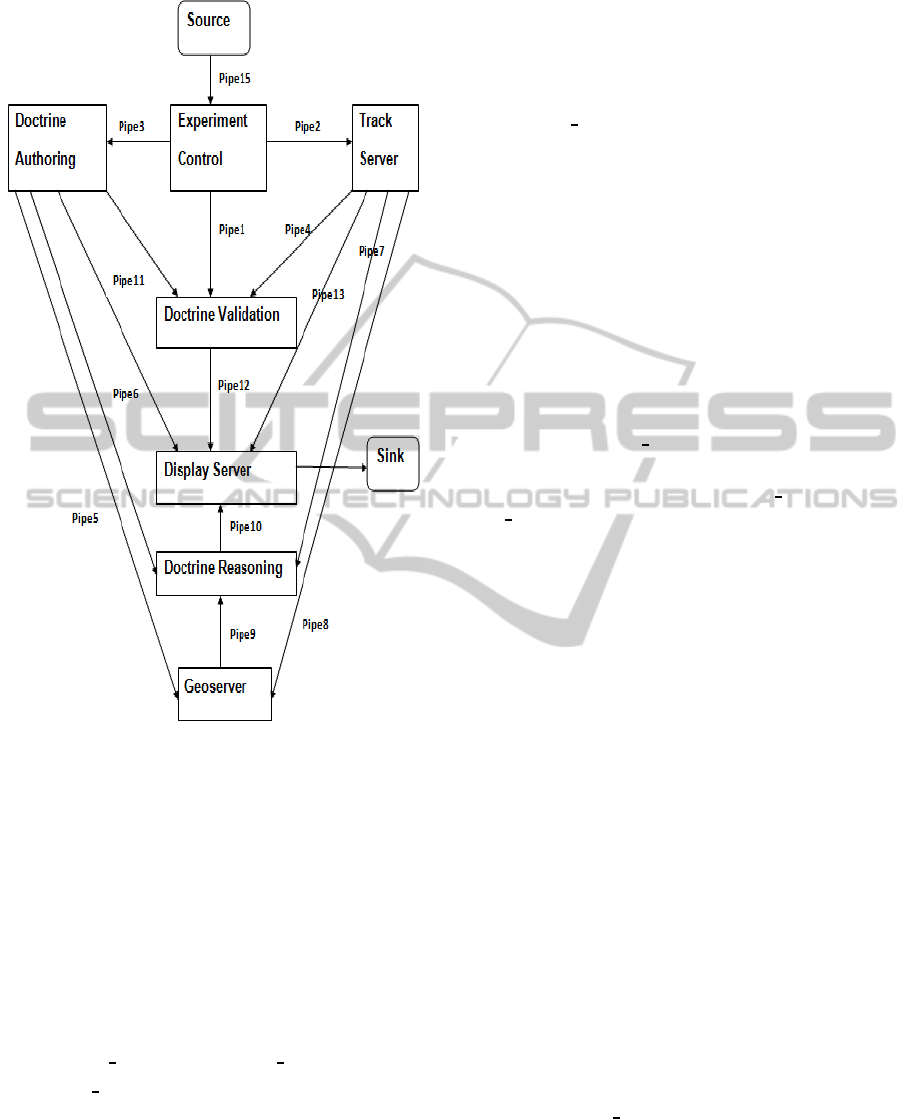
Figure 2: Aegis system architecture represented in ACME

Studio.

• ACME+ Description

Using our proposed constructs of functional

dependency, we give below examples of ACME+

descriptions. For the sake of brevity, we content

ourselves with giving ACME+ descriptions of only

two components of Aegis system. The overall

architecture description of the Aegis Weapon System

in ACME+ is available online at:

http://web.njit.edu/∼mili/AegisArch.txt.

We present ACME+ descriptions of the two compo-

nents Display

Server and Doctrine Authoring.

1. Display

Server operates in a single process (R) re-

quiring all data from its input ports to display the

results on its output port.

Component Display_Server {

Port inPort0; Port inPort1;

Port inPort2;Port inPort3;

FunDep = {R(

Input(AllOf(Synchronous(inPort0; inPort1;

inPort2; inPort3)));

Output(outPort);

Properties(procTime=1;thruPut=0.4;failProb=0.3)

)}};

2. The second example concerns the component

Doctrine Authoring which operates in a single

task (R). Its output ports send simultaneously du-

plicate information.

Component Doctrine_Authoring {

Port inPort; Port outPort0;

Port outPort1; Port outPort2; Port outPort3;

FunDep= {R(

Input(inPort);

Output(Duplicate(Simultaneous(outPort1;

outPort0;outPort2; outPort3)));

Properties(procTime= 0.7;thruPut=0.2;

failProb=0.2))}};

• Inductive Rules

The compiler generates the following Mathematica

equations for Display Server:

Within Component Display

Server. Dis-

play Server input ports are related with AllOf

relation. Then, if we refer to equation 2, we can

write:

DisplayServer.outPort.RT = Max(

DisplayServer.inPort0.RT;

DisplayServer.inPort1.RT;

DisplayServer.inPort2.RT;

DisplayServer.inPort.RT)+

DisplayServer.R1. procTime

(14)

With reference to equation 5, we can write:

DisplayServer.outPort.TP = Min(

DisplayServer.R.thruPut;

∑

i=0

(C.inPort

.TP))

(15)

With reference to equation 8, we can write:

DisplayServer.outPort.FP = 1−

(1− DisplayServer.R. failProb)×

(1−

∏

i=0

DisplayServer.inPort

.FP)

(16)

Between Display

Server and Connectors. When-

ever a component port is attached to a connector role,

the attribute values are passed forward from the out-

put port to the source role. Hence, we write:

DisplayServer.inPort0.RT = Pipe13.toRole.RT

(17)

ComputingAttributesofSoftwareArchitectures-AStaticMethodandItsValidation

DisplayServer.inPort1.RT = Pipe10.toRole.RT

(18)

DisplayServer.inPort2.RT = Pipe12.toRole.RT

(19)

DisplayServer.inPort3.RT = Pipe11.toRole.RT

(20)

DisplayServer.outPort.RT = Pipe14. fromRole.RT

(21)

The compiler generates the following Mathematica

equations for Doctrine Authoring :

Within Component Doctrine

Authoring. Doc-

trine

Authoring has only one input port, then the re-

sponse time of each outPort

, i = 0..3, is equal to the

sum of its processing time and the response time of

its input port. We write:

DoctrineAuthoring.outPort

.RT =

(DoctrineAuthoring.R1. procTime+

DoctrineAuthoring.inPort.RT);i = 0..3

(22)

The throughput of each outPort

, i = 0..3, is

equal to the minimum between its throughput and the

throughput of its input port. We write:

DoctrineAuthoring.outPort

.TP =

Min(DoctrineAuthoring.R.thruPut;

C.inPort.TP);i = 0..3

(23)

In order for a computation that is initiated at

DoctrineAuthoring.outPort

i = 0..3, to succeed,

component Doctrine Authoring has to succeed, and

the computation initiated at its input port has to suc-

ceed. Assuming statistical independence, the proba-

bility of these simultaneous events is the product of

probabilities. Hence, we write:

DoctrineAuthoring.outPort

.FP =

1− (1− DoctrineAuthoring.R. failProb)×

(1− DoctrineAuthoring.inPort.FP);i = 0..3

(24)

Between Doctrine

Authoring and Connectors.

Whenever a component port is attached to a connec-

tor role, the attribute values are passed forward from

the output port to the source role. Hence, we write:

DoctrineAuthoring.inPort.RT = Pipe0.toRole.RT

(25)

DoctrineAuthoring.outPort0.RT = Pipe5. fromRole.RT

(26)

DoctrineAuthoring.outPort1.RT = Pipe3. fromRole.RT

(27)

DoctrineAuthoring.outPort2.RT = Pipe6. fromRole.RT

(28)

DoctrineAuthoring.outPort3.RT = Pipe11. fromRole.RT

(29)

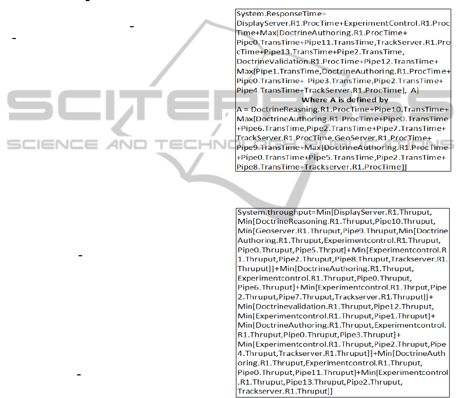
• System Properties

To determine the response time, the throughput and

the failure probability of the system, we use Math-

ematica to solve the system of equations derived by

the compiler taking as unknown Datasink.input.RT,

Datasink.input.TP and Datasink.input.FP respec-

tively. Figure 3 depicts the system response time, ﬁg-

ure 4 depicts the system throughput and ﬁgure 5 de-

picts the system failure probability.

Figure 3: Aegis response time as function of its components

and connectors response time.

Figure 4: Aegis throughput as function of its components

and connectors throughput.

• Reliability Sensitivity Analysis

We propose to analyze the sensitivity of the Aegis

system relatively to the reliability. Thus, we propose

to use Mathematica to calculate the derivative of the

system failure probability with respect to the failure

probability of each one its components / connectors.

The derivative of the formula is deﬁned by the equa-

tion 30, where C

represents component i.

ENASE2015-10thInternationalConferenceonEvaluationofNovelSoftwareApproachestoSoftwareEngineering

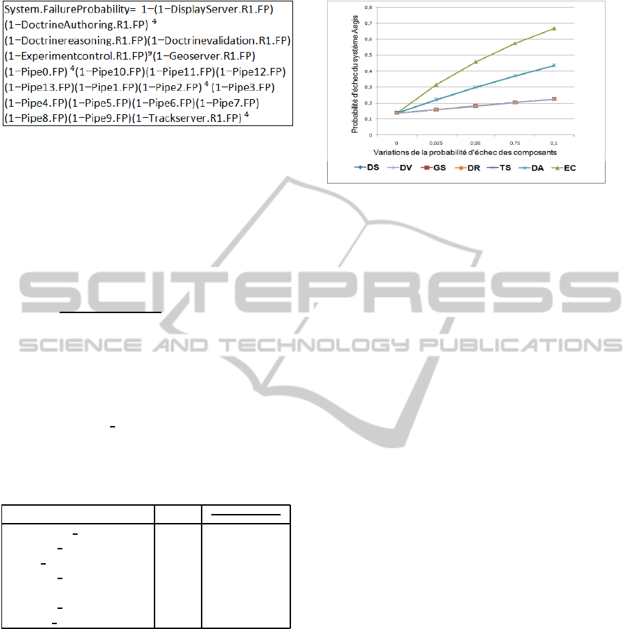
Figure 5: Aegis failure probability as function of its com-

ponents and connectors failure probability.

In this example, we assume that all connectors

have a low probability of failure equal to 0.001 and

we propose to determine the component representing

the reliability bottleneck. So, for each component of

Aegis, we calculate the derivative deﬁned in equation

30.

∂System.FailProb

∂C

.FailProb

;i = 1, 2, ..., n (30)

In table 1, the components are ordered by decreas-

ing order of their derivatives values. The component

having the largest value of the derivative is the one

that most affects the reliability of the system, it is the

bottleneck of the system. More speciﬁcally, the com-

ponent Experiment

control is on the top of the list,

showing that it has an impact on the overall system

reliability.

Table 1: Reliability sensitivity analysis.

Composant C C.FP

∂System.FailProb

∂C.FP

Experiment Control(EC) 0.007 7.813

Doctrine Authoring(DA) 0.004 3.462

Track Server(TS) 0.006 3.469

Doctrine Reasoning(DR) 0.008 0.869

Geoserver(GS) 0.009 0.869

Doctrine Validation(DV) 0.005 0.866

Display Server(DS) 0.003 0.864

To check on our approach of sensitivity analysis

of Aegis system, we study the effect of variations of

components reliabilities to identify points in the ar-

chitecture where the variation has a higher impact on

the property of the whole system. Thus, we vary the

probability of failure of each component of the Aegis

system (variation of 0.025) and calculate the failure

probability of the system by keeping ﬁxed the val-

ues of failure probability of other components. The

same variations of failure probabilities values are per-

formed for all components.

The graph in ﬁgure 6 depicts the failure proba-

bility of the overall system according to variations of

0.025 on components failure probabilities.

Figure 6: Reliability sensitivity analysis.

For the readability of the results, in the graphic’s

caption, from the left to the right, components are

ordered from the lower to the higher increase of the

impact on the overall system reliability. The graph

clearly shows that the component Experimentcontrol

has the highest impact, representing then, the bottle-

neck of the system. Hence, we note the compliance of

conclusions drawn from the graph compared to those

found by our approach.

7.2 Analysis of Aegis System by

Simulation

In order to simulate Aegis system, we have ﬁrst cod-

iﬁed the architecture of the whole system using an

(M × N) matrix which we denote by arch. M rep-

resents the number of system connectors and N is re-

ferred to the number of system components. This ma-

trix describes the links between components and con-

nectors. The intersection of a line i with a column

j in arch matrix indicates whether the connector i is

connected by its source role to the component j, is

connected by its destination role to the component j

or is not connected to this component.

Functional dependency relations (AllOf, AnyOf,

MostOf), expressing links between input ports of the

component, are also codiﬁed using relation matrix.

Each column j of the relation matrix describes which

connectors have to complete their transmissions in or-

der to let component j proceed.

In order to compare the results found by our analy-

sis tool ACME+ and those found by the simulation

method, we proceed as follows:

1. we generate random values of components and

connectors non-functional properties,

2. we use the formula found by our ACME+ analysis

tool to calculate the property of the whole system.

Let’s recall that this formula expresses the prop-

erty of the overall system based on the properties

ComputingAttributesofSoftwareArchitectures-AStaticMethodandItsValidation

of components and connectors,

3. we execute the simulation using the values of

components and connectors properties which are

generated in step 1,

4. we store the results found by ACME+ tool and by

simulation method,

5. Finally, we compare the obtained results.

The whole process is applied to each one of the qual-

ity attributes: response time, throughput and reliabil-

ity. It is repeated a hundred times in order to validate

our inductive reasoning.

• Response Time Simulation

To calculate the system response time by the simu-

lation method, we have used an array of structure,

which we denote by Exec. It stores for each compo-

nent and each connector respectively his ”execution

time” and his ”transmission time”, its ”state” de-

scribing the state of the component or the connec-

tor: ”waiting”, ”finished” or in ”execution”, ”time”

expressing the remaining time for the component or

connector to terminate and go to the state ”finished”.

Initially, for every element of Exec (corresponding to

a component or connector), ﬁelds ”execution time”

and ”transmission time” are initialized to correspond-

ing values randomly generated, the ﬁeld ”state” is set

to ”waiting”, the value of the ﬁeld ”time” is set to the

value of the execution time / transmission time of the

component / connector.

In order to simulate the performance of the Aegis

system, we start by assuming that the component

Datasource starts execution and all other components

are pending. We initialize the value of a clock to 0.

We iterate over the array of structure Exec. In each

iteration, the value of clock is incremented by 1 and

at the same time:

• the ﬁeld ”time” of components and connectors in

execution are decremented by 1,

• components and connectors that have ﬁnished,

have their states changed to ”finished” ,

• check which components or connectors must be

triggered and change their states to ”execution”.

This requires consulting matrices arch and

relation to verify the links between components

and connectors.

The system response time is the value of the clock

when the states of all components and connectors are

changed to ”finished”.

• Throughput Simulation

To calculate the throughput of the system by the

method of simulation, we have used an array of

structure Exec that stores for each component / con-

nector their throughput values randomly generated,

their ”state” describing the state of the component /

connector: ”waiting”, ”finished” or in ”execution”,

”time” representing the time remaining to complete

and pass the state ”finished”, ”amount”, the amount

of information processed or communicated by the

component or the connector. The amount of an archi-

tectural element depends on the amount of informa-

tion received and on its throughput. In order to sim-

ulate the execution of the Aegis system, we start by

assuming that the component Datasource starts ex-

ecution and all other components are pending. Ini-

tially the ”amount” of each component and connector

is set to 0, the ”time” of each component is set to its

execution time and that of each connector is initial-

ized to its transmission time. Except the ﬁrst compo-

nent who starts its execution, its ”amount” is set to its

throughput.

We iterate over the array of structure Exec. In each

iteration:

• ”time” of components and connectors in execu-

tion are decremented by 1,

• components and connectors that have ﬁnished,

have their states changed to ”finished”,

• check which components or connectors must be

triggered and change their states to ”execution”

and change their ﬁelds ”amount” to the amount

of data that they can treat or emit. This requires

consulting matrices arch and relation to verify the

links between components and connectors. The

”amount” of an architectural element is equal to

the minimum between the ”amount” received and

its throughput.

The system throughput will be the value of ”amount”

emitted by the last component of the architecture that

was executed.

• Failure Probability Simulation

To determine the reliability of the system by the

method of simulation, we used an array of struc-

ture that stores for each component / connector

his ”probabilityof failure”, its ”state” (”waiting”,

”finished”, ”execution”), the ”time” remaining to ﬁn-

ish and move on to the state ”finished” and ”run”

which indicates whether the component / connector

succeeds or fails. We generate random values of com-

ponents and connectors probabilities of failure. We

also randomly determine if the architectural element

fails or succeeds the current execution, according to

its probability of failure. The overall system succeeds

or fails based on the failure or the success of its com-

ponents and connectors. We iterate over the array of

structure Exec. In each iteration:

ENASE2015-10thInternationalConferenceonEvaluationofNovelSoftwareApproachestoSoftwareEngineering

• the ﬁeld ”time” of components and connectors in

execution are decremented by 1,

• components and connectors that have ﬁnished,

have their states changed to ”finished”,

• check which components or connectors must be

triggered and change their states to ”execution”.

This requires consulting matrices arch and

relation to verify the links between components

and connectors.

• verify which components and which connectors

have succeeded or have failed and update their

corresponding values of ”run”.

The success or the failure of the overall system is de-

termined by the success or the failure of the last ex-

ecuted component. The steps already described are

repeated several times (100 or 200 times) and each

time, we determine whether the system succeeds or

fails. We then calculate the probability of failure of

the system as the quotient of the number of failures

by the total number of tests.

7.3 Comparison of Analysis Results

We have analyzed Aegis system using two ap-

proaches: simulation and ACME+ tool. We have run

many tests, in each test we generate random values

of components and connectors properties. Then, we

run our analysis tool ACME+ on these values in order

to calculate properties of the whole system. We also

run the simulation and ﬁnally, we compare the results

found by the two methods.

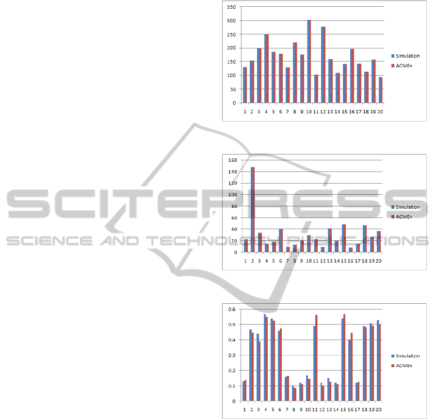
To visualize the difference between the obtained

results, we propose to represent the analysis results in

bar charts graphics which plot Aegis properties com-

puted by ACME+ tool and by simulation in each test.

Graphics shown by ﬁgures 7, 8, 9 depicts an exam-

ple of 20 tests done to compare respectively response

time, throughput and failure probability values found

by simulation approach and by our ACME+ tool.

Figures 7, 8 show that the analysis of the Aegis

system by simulation and ACME+ tool generates

equal values of response time and throughput prop-

erties. However, ﬁgure 9, relative to failure probabil-

ity property, shows close results. Hence, these results

claim the validity of our inductive reasoning.

8 CONCLUSION

In this paper, we propose an ADL based formal

method for representing and reasoning about system

non-functional attributes at the architectural level. We

Figure 7: Aegis response time values found by simulation

and ACME+.

Figure 8: Aegis throughput values found by simulation and

ACME+.

Figure 9: Aegis failure probability values found by simula-

tion and ACME+.

aim to automatically analyze performance and reli-

ability of system architecture from performance and

reliability of its components and connectors. For

these reasons, we propose ACME+ as an extension of

Acme ADL, and discuss the development and opera-

tion of a compiler that compiles architectures written

in ACME+ ADL to generate equations that character-

ize non functional attributes of software architectures.

We then conduct a sensitivity analysis on the results,

to determine existent bottlenecks that most affect the

performance and the reliability of the system. This

will help architects to identify components and con-

nectors that need urgent attention to be improved in

order to ameliorate system quality.

ComputingAttributesofSoftwareArchitectures-AStaticMethodandItsValidation

Our work can be characterized by the following

attributes, which set it apart from other work on ar-

chitectural analysis.

• from a software architectural speciﬁcation it is

quite simple to derive an ACME+ textual descrip-

tion thanks to its expressiveness.

• we propose to estimate the non-functional prop-

erties directly from an architectural description to

avoid problems occurred when using a mathemat-

ical models. In fact, the transformation of soft-

ware architecture to a mathematical model, im-

posed by the analytical approaches, limits their

capacities of analysis which depends on the used

model.

• our analysis approach can be applied to any sys-

tem that can be described by components and con-

nectors for any architectural style (client/server,

pipes and ﬁlters, etc.) unlike Acme-based ap-

proach, presented in (Spitznagel and Garlan,

1998), which is limited to client/server systems

analysis.

• system analysis must deal with various quality at-

tributes to enable a better understanding of the

strengths and weaknesses of complex systems

(Dobrica and Niemelae, 2002). Thus, unlike ap-

proaches found in the literature, which analyze ei-

ther performance or reliability quality attributes,

it is possible with the same ACME+ speciﬁcation

of a software system to analyze both performance

and reliability. It is also possible to extend anal-

ysis to other quality attributes that can be induc-

tively derived such as availability, maintainability,

etc.

• our approach is supported by an automated tool.

The user can perform many different experi-

ments by analyzing the software architecture and

modifying the components and connectors non-

functional properties values or changing the soft-

ware topology to get better performances before

iterating the process again. It is then very easy

to perform many ”what-if” experiments, changing

parameters or structure of the model to see what

the result is.

Among the extensions we envision for this work, we

cite: the analysis of other quantitative non functional

attributes and to investigate more profoundly archi-

tecture styles and dynamic architectures.

REFERENCES

(December 2005). Wr2fdr. http://www.cs.cmu.edu/∼able/

wright/wr2fdr

bin.tar.gz.

Allen, R. and Garlan, D. (1996). A case study in architec-

tural modeling: The aegis system. In In Proceedings

of the 8th International Workshop on Software Speci-

ﬁcation and Design, pages 6–15.

Aquilani, F., Balsamo, S., and Inverardi, P. (2001). Per-

formance analysis at the software architectural design

level. Perform. Eval., 45(2-3):147–178.

Balsamo, S., Bernardo, M., and Simeoni, M. (2002). Com-

bining stochastic process algebras and queueing net-

works for software architecture analysis. In Workshop

on Software and Performance, pages 190–202.

Bass, L., Clements, P., and Kazman, R. (1998). Software

Architecture in Practice. Addison Wesley Longman

Publishing Co., Inc., Boston, MA, USA.

Bosch, J. (1999). Design and use of industrial software ar-

chitectures. In Proceedings of Technology of Object-

Oriented Languages and Systems.

Cheung, R. (1980). A user-oriented software reliability

model. IEEE Trans. on Software Engineering, 6:118–

125.

Denning, P. and Buzen, J. (1978). The operational analysis

of queueing network models. ACM Computing Sur-

veys, 10:225–261.

Dobrica, L. and Niemelae, E. (2002). A survey on software

architecture analysis methods. IEEE Transactions on

Software Engineering, 28:638–653.

Franco, J., Barbosa, R., and Rela, M. (2012). Automated re-

liability prediction from formal architectural descrip-

tions. In WICSA/ECSA, pages 302–309.

Giannakopoulou, D., Kramer, J., and Cheung, S. (1999).

Behaviour analysis of distributed systems using the

tracta approach. Journal of Automated Software Engi-

neering, 6(1):7–35.

Gokhale, S. S. (2007). Architecture-based software reliabil-

ity analysis: Overview and limitations. IEEE Trans.

Dependable Sec. Comput., 4(1):32–40.

Goseva-Popstojanova, K. and Trivedi, K. (2001).

Architecture-based approach to reliability assess-

ment of software systems. Journal of Performance

Evaluation, 45(2-3):179–204.

Kompanek, A. (1998). Acmestudio user’s manual.

Krishnamurthy, S. and Mathur, A. P. (1997). On the estima-

tion of reliability of a software system using reliabil-

ities of its components. In Proceedings of the Eighth

International Symposium on Software Reliability En-

gineering, ISSRE ’97, pages 146–155.

Kwiatkowska, M., Norman, G., and Parker, D. (2009).

Prism: Probabilistic model checking for performance

and reliability analysis. ACM SIGMETRICS Perfor-

mance Evaluation Review, 36(4):40–45.

Medvidovic, N. and Taylor, R. (2000). A classiﬁcation and

comparison framework for software architecture de-

scription languages. IEEE Transactions on Software

Engineering, 11(1):70–93.

Shooman, M. (1976). Structural models for software reli-

ability prediction. In Proceedings of the 2Nd Inter-

national Conference on Software Engineering, ICSE

’76, pages 268–280.

Spitznagel, B. and Garlan, D. (1998). Architecture-based

performance analysis. In Proceedings of the 1998

Conference on Software Engineering and Knowledge

Engineering, pages 146–151.

ENASE2015-10thInternationalConferenceonEvaluationofNovelSoftwareApproachestoSoftwareEngineering