
Inferring Geo-spatial Neutral Similarity from Earthquake Data using
Mixture and State Clustering Models
Avi Bleiweiss
Platform Engineering Group, Intel Corporation, Santa Clara, U.S.A.
avi.bleiweiss@intel.com
Keywords:
Earthquake, Seismic, Mixture Model, Expectation-maximization, Hidden Markov Model, Clustering.
Abstract:
Traditionally, earthquake events are identified by prescribed and well formed geographical region boundaries.
However, fixed regional schemes are subject to overlook seismic patterns typified by cross boundary relations
that deem essential to seismological research. Rather, we investigate a statistically driven system that clus-
ters earthquake bound places by similarity in seismic feature space, and is impartial to geo-spatial proximity
constraints. To facilitate our study, we acquired hundreds of thousands recordings of earthquake episodes that
span an extended time period of forty years, and split them into groups singled out by their corresponding
geographical places. From each collection of place affiliated event data, we have extracted objective seismic
features expressed in both a compact term frequency of scales format, and as a discrete signal representation
that captures magnitude samples in regular time intervals. The distribution and temporal typed feature vectors
are further applied towards our mixture model and Markov chain frameworks, respectively, to conduct cluster-
ing of shake affected locations. We performed extensive cluster analysis and classification experiments, and
report robust results that support the intuition of geo-spatial neutral similarity.
1 INTRODUCTION
Modern seismological exploration of disseminating
earthquake sites and magnitudes rests on both the
advancement in instrumental seismometry and the
analysis of macroseismic effects, including geologi-
cal structures, population, and the landscape (Hough,
2014). To describe the severity of shaking, seismic ef-
fects are commonly assigned an intensity scale set by
different yet fairly correlated standards, traditionally
in the range of one to ten. In recent years, the develop-
ment of methods to quantitatively and objectively an-
alyze scale data, coupled with the emerging of online
systems to generate unprecedented volumes of both
real-time and archival earthquake data, had sparked
renewed interest in research to assess global seismic
intensity distribution. One indispensable resource for
practitioners in the field is the United States Geolog-
ical Survey (USGS, 2004) science organization, fully
devoted to furnish impartial information on the health
of our ecosystem. Amongst the many services, USGS
provides a large web based repository of geo-spatially
rich data for expressing earthquake events that are dy-
namically collected as they occur, and furthermore al-
lows for this knowledge base to be programmatically
accessible for software development. Figure 1 shows
a high level, distributed earthquake scale around the
globe, based on USGS data we acquired that repro-
duces an extent of four decades, from 1975 till 2014.
In our work, we investigate a discovery (Rajara-
man and Ullman, 2011) method that extracts a statisti-
cal relation model of earthquake bound geographical
locations from a large data set of hundreds of thou-
sands of recorded seismic events, and incorporates
both information retrieval (Manning et al., 2008) and
unsupervised machine learning (Duda et al., 2001)
techniques. Information retrieval (IR) is rapidly be-
coming the dominant form of data source access.
Amongst multitude disciplines, IR encompasses the
field of grouping a set of documents that enclose non
structured content, to behave similarly with respect
to relevance to information needs. Our work closely
leverages IR practices by realizing a seismic bound
place after a text document, composed of a collection
of intensity scales and represented in a compact his-
togram of term frequencies format. For a broader con-
text, we contrast this distribution feature form with a
classic, discrete seismic signal constructed of a series
of shake magnitudes over time that spans a course
of several tens of years. Furthermore, we are inter-
ested in uncovering objectively the underlying cluster
nature of hundreds of geographical sites, without re-
5
Bleiweiss A..
Inferring Geo-spatial Neutral Similarity from Earthquake Data using Mixture and State Clustering Models.
DOI: 10.5220/0005347500050016
In Proceedings of the 1st International Conference on Geographical Information Systems Theory, Applications and Management (GISTAM-2015), pages
5-16
ISBN: 978-989-758-099-4
Copyright
c
2015 SCITEPRESS (Science and Technology Publications, Lda.)
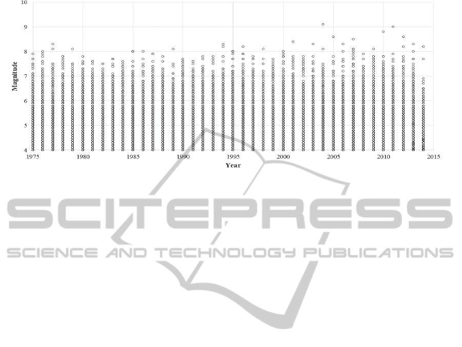
Figure 1: Earthquake events: showing magnitude scale as a function of time, tracking forty years from 1975 till 2014.
sorting to any prior knowledge of the erupting phys-
ical location, nor to constraining geo-spatial proxim-
ity as prescribed by the Flinn-Engdahl regionalization
scheme (Young et al., 1995). To this extent, we use
both finite mixture (Mclachlan and Peel, 2000) and
Markov chain (Rabiner, 1989) models, recognized for
providing effective and formal statistical framework
to cluster high dimensional data of continuous nature.
Finite mixture models are widely used in the field
of cluster analysis (Fraley and Raftery, 2002) (Fra-
ley and Raftery, 2007), and apply to a growing ap-
plication space including web content search, gene
expression linking, and image segmentation. They
form an expressive set of classes for multivariate den-
sity estimation, and the entire observed data set of
scale histograms is represented by a mixture of ei-
ther continuous or discrete, parametric distribution
functions. An individual distribution, often referred
to as a component distribution, constitutes thereof a
cluster. Traditionally, the likelihood paradigm pro-
vides a mechanism for estimating the unknown pa-
rameters of the mixture model, by deploying a method
that iterates over the maximum likelihood. One of
the more broadly used and well behaved technique
to guarantee process convergence is the Expectation-
Maximization (EM) algorithm (Dempster et al., 1977)
that scales well with increased data set size. Upon
completion, the likelihood function reflects the con-
formity of the model to the incomplete observed data.
While not immediately applicable to our work, note-
worthy is the research that further extends the empiri-
cal likelihood paradigm to a model, whose component
dimension is unknown. Hence, both model fitting and
selection must be determined from the data simultane-
ously, by using an approximation based on any of the
Akaike Information Criterion (AIC) (Akaike, 1973),
the Bayesian Information Criterion (BIC) (Schwarz,
1978), or the sum of AIC and BIC plus an entropy
term (Ngatchou-Wandji and Bulla, 2013).
The discrete Hidden Markov Model (HMM)
(Baum and Petrie, 1966) (Rabiner, 1989) is a prob-
abilistic framework that formalizes a reasoning about
a series of observations over time, to recover a set of
states. The model is extensively used in many appli-
cation domains including speech recognition, biolog-
ical sequence analysis, and stochastic natured finan-
cial economics. HMM is described by a set of param-
eters that are estimated to maximize the probability
of an observation. Much like the mixture model, it
employs the maximum likelihood estimation princi-
pal and commonly uses the Baum-Welch algorithm
(Baum, 1972), an analog to the EM method. In our
work, we characterize a time progression of earth-
quake events, occurring in a prescribed geographi-
cal location, as a discrete seismic signal comprised of
shake scale samples. A seismic signal thus forms an
observation vector, and a collection of these temporal
feature vectors are applied to HMM, deriving for each
a log-likelihood measure. Unlike the mixture model,
the grouping of observation vectors in HMM is not
implicit, hence we follow HMM to perform hierarchi-
cal agglomerative clustering (Manning and Schutze,
2000) (Johnson, 1967) on log-likelihood values.
The main contribution of our work is a novel, sta-
tistically drivensystem that combines IR and unsuper-
vised learning techniques to discover instinctive clus-
ter patterns from presumed unlabeled seismic data,
and best match earthquake bound geographical loca-
tions by objective similarity in feature space. In con-
trast to a more constraining approach that prescribes
physical regionalization boundaries. The remainder
of this paper is organized as follows. We overview
the motivation for selecting seismic feature represen-
tations, leading to our compact formats of intensity
GISTAM2015-1stInternationalConferenceonGeographicalInformationSystemsTheory,ApplicationsandManagement
6

scale distribution and a time series signal, in section
2. Section 3 reviews algorithms and provides the-
ory to multivariate cluster analysis, discussing both
the normal mixture model and Markov chain foun-
dations, and the role of their respective EM method
in estimating model parameters. Whereas in section
4, we present our evaluation methodology of seismic
cluster analysis and classification, and report quanti-
tative results of our experiments. We conclude with a
discussion and future prospect remarks, in section 5.
2 SEISMIC FEATURES
We acquired seismic data from the USGS (USGS,
2004) science organization. USGS provides real-time
earthquake data in a well-structured format, GeoJ-
SON (GeoJSON, 2007), readily parsed by most pro-
gramming languages. GeoJSON uses the popular
JavaScript Object Notation (JSON) to encode a di-
verse set of geographic data structures. A GeoJSON
object may represent any of a geometry, a feature or a
collection of features. Typically, an earthquake event
is characterized by a geometrical bounding box and
a set of seismic features (Table 1). The three dimen-
sional volume of eruption is defined by the minimum
and maximum extent of each of the longitude, lati-
tude, and depth attributes. An event specifies a rather
extensive set of seismic properties, although many of
them appear either unavailable or partially missing in
the data frames we gathered. Most relevant features
to our work include the magnitude, magnitude type,
place, and time. The magnitude value is measured
and recorded by a seismograph that responds to dis-
tinct seismic waves traveling through the ground, who
are excited by relative motion of the earth. Whereas
magnitude type identifies the method or algorithm to
calculate the scale of the event. Most commonly used
scales comprise of local (M
l
), also referred to the
Richter scale, surface-wave (M
s
), body-wave (M
b
),
and moment (M
w
) metrics. Moment scale is directly
related to the faulting process and is considered a
more consistent measure of earthquake size, unlike
the rest that are accuracy limited by an upper bound.
Nonetheless, all magnitude types yield approximately
the same value for a given earthquake event. The
place property is a named geographic location closest
to the event, either a city or a region enumerated in the
Flinn-Engdahl seismic and geographical, globe parti-
tioning scheme (Flinn-Engdahl, 2000), along with the
time of a shake occurrence, reported in milliseconds.
Our seismic dataset comprises several hundreds of
thousands earthquake events that track an extended
time period of several tens of years. The process of
extracting features from this large seismic collection
proceeds in several stages. First, we split the dataset
into groups, each embedding all event occurrences
in an identical place or region, chronologically. Our
transformed dataset represents now a compilation of
distinct places drawn out from our raw data, and totals
several thousands data points. Let P = {p
1
, p
2
, ..., p
n
}
be our observed, place subjected seismic data, with
each place data point, p
i
, retaining a different event
count. Next, we derive from each data sample, p
i
, two
domain feature vectors to provide for unified dimen-
sionality. An unnormalized, scale distribution vector
D ∈ N
|V|
, with |V| the number of possible magnitude
values, and a time series vector S ∈ R
d
of a sampling
dimensionality d.
Table 1: Features extracted from a GeoJSON object that
describes geometry and selected seismic properties of an
earthquake event. Showing for each value range and units.
(a) Bounding Box.
Dimension Range Units
longitude [−180.0
◦
, +180.0
◦
] degrees
latitude [−90.0
◦
, +90.0
◦
] degrees
depth [0, 1000] kilometer
(b) Seismic Properties.
Feature Range Units
mag [−1.0, 10.0] scale
mag type M
l
, M
s
, M
b
, M
w
string
place Flinn-Engdahl region string
time date-time milliseconds
D formalizes a term frequency description that as-
signs each vector element a count of unique mag-
nitude occurrences, accumulated in the events pre-
scribed to a place data point, p
i
. This is modeled af-
ter the bag of words (Baeza-Yates and Ribeiro-Neto,
1999) representation, a simple and one of the more ef-
fective text retrieval methods, founded on the premise
that the respective order of events to emerge in a loca-
tion, is ignored. In our work, we tend to events who
record a scale in the [4.0, 9.9] range and sampled in
0.1 increments, hence |V|, the dimensionality of D,
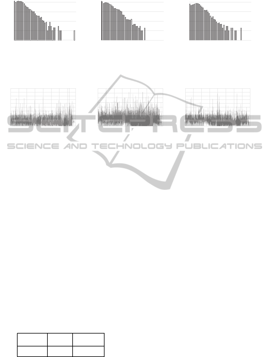
amounts to 60 elements. Figure 2 outlines scale dis-
tribution feature vectors extracted from three distinct,
place data points. The location compact format of
bag of scale words is passed on to our mixture model
to perform seismic place clustering, and follows ef-
ficient similarity calculations, directly from the well
known Vector Space Model (Salton et al., 1975).
The raw, time series vector we extract is an irreg-
ular periodicity formulation of magnitudes, dispersed
InferringGeo-spatialNeutralSimilarityfromEarthquakeDatausingMixtureandStateClusteringModels
7
0.1
1
10
100
1000
4 4.5 5 5.5 6 6.5 7 7.5 8 8.5
9
Frequency
Magnitude
(a) Honshu, Japan.
0.1
1
10
100
1000
4 4.5 5 5.5 6 6.5 7 7.5 8 8.5
9
Frequency
Magnitude
(b) Fiji region.
0.1
1
10
100
1000
4 4.5 5 5.5 6 6.5 7 7.5 8 8.5
9
Frequency
Magnitude
(c) Kuril Islands.
Figure 2: Scale distribution feature vector: showing in log scale the number of magnitude occurrences extracted from events
associated with a place data point, for three geographical locations.
4
4.5
5
5.5
6
6.5
7
7.5
8
8.5
9
1975 1980 1985 1990 1995 2000 2005 2010
2015
Magnitude
Time
(a) Honshu, Japan.
4
4.5
5
5.5
6
6.5
7
7.5
8
1975 1980 1985 1990 1995 2000 2005 2010
2015
Magnitude
Time
(b) Fiji region.
4
4.5
5
5.5
6
6.5
7
7.5
8
8.5
9
1975 1980 1985 1990 1995 2000 2005 2010
2015
Magnitude
Time
(c) Kuril Islands.
Figure 3: Time series feature vector: resampled irregular raw signal using the year-week sampling mode, for three geograph-
ical locations. A sample of no event is assigned a zero magnitude.
sequentially along the course of our event capturing
time frame of forty years. S is then further resampled
with regular time intervals consisting of year-week,
monthly and bi-monthly formats, thus leading to a
time series feature vector of dimensionality depicted
in Table 2. Our year-week sample index, [0, 53], fol-
lows the US rule, and for a place of multiple events,
excited in the same week, we compute a weekly mean
of all magnitudes to ensure a single scale is identified
with a week. Whereas a week of no event defaults
to the value of zero intensity. The monthly and bi-
monthly sampling modes arise from a direct decima-
tion of the year-week signal by a factor of four and
eight, respectively. Time series vectors, resampled in
the year-week mode for three geographical places are
further illustrated in Figure 3. Subsequently, we use a
hidden Markov chain (HMM) to model the durational
and spectral variability of our generated seismic sig-
nal, S, that constitutes an observation vector.
Table 2: Time series vector: listing uniform resampling
modes and corresponding dimensionality.
Year-Week Monthly Bi-Monthly
2120 530 265
3 PLACE CLUSTERING
Clustering procedures based on finite mixture mod-
els provide a flexible approach to multivariate statis-
tics. They become increasingly preferred over heuris-
tic methods, owing to their robust mathematical ba-
sis. Mixture models standout in admitting clus-
ters to directly identify with the components of the
model. To model our system probability distribu-
tion of scale count features, we deploy the well es-
tablished, Normal (Gaussian) Mixture Model (GMM)
(Mclachlan and Basford, 1988) (Mclachlan and Peel,
2000), known for its parametric, probability density
function that is represented as a weighted sum of
Gaussian component densities. GMM parameters are
estimated from our incomplete training data, com-
posed of bags of intensity scale words, using the
iterative Expectation-Maximization (EM) (Dempster
et al., 1977) algorithm. Correspondingly, for our
place bound, seismic signal features we exploit the
Hidden Markov Model (HMM) (Baum and Petrie,
1966) (Rabiner, 1989), using the Baum-Welch algo-
rithm (Baum, 1972) to repeatedly recalibrate model
parameters, and follow this process to construct an ag-
glomerative hierarchy of seismic aware clusters, em-
ploying an efficient dynamic tree cutting technique.
GISTAM2015-1stInternationalConferenceonGeographicalInformationSystemsTheory,ApplicationsandManagement
8

3.1 Normal Mixture Model
Let X = {x
1
, x
2
, ..., x
n
} be our observed collection of
seismic bound places, each represented as an intensity
scale, term frequency vector I ∈ N
d
. An additive mix-
ture model, defines a weighted sum of k components,
whose density function is formulated by equation 1:
p(x|Θ) =
k
∑
j=1
w
j
p
j
(x|θ
j
), (1)
where w
j
is a mixing proportion, signifying the prior
probability that an observed place x, belongs to the
j
th
mixture component, or cluster. Mixing weights,
satisfy the constraints
∑
k
j=1
w
j
= 1, and w
j
≥ 0. The
component probability density function, p
j
(x|θ
j
), is
a d-variate distribution, parameterized by θ
j
. Most
commonly, and throughout this work, p
j
(x|θ
j
) is the
multivariate normal (Gaussian) density (equation 2),
characterized by its mean vector µ
j
∈ R
d
and a co-
variance matrix Σ
j
∈ R
dxd
. Hence, θ
j
= (µ
j
, Σ
j
), and
the mixture parameter vector Θ = {θ
1
, θ
2
, ...., θ
k
}.
1
(2π)
d
2
p
|Σ
j
|
exp(−
1
2
(x− µ
j
)
T
Σ
−1
j
(x− µ
j
)) (2)
Seismic places, distributed by mixtures of multi-
variate normal densities, are members of clusters that
are centered at their means, µ
j
, whereas the cluster ge-
ometric feature is determined by the covariance ma-
trix, Σ
j
. For efficient processing, our covariance ma-
trix is diagonal, Σ
j
= diag(σ
2
j1
, σ
2
j2
, ..., σ
2
jd
), and thus
clusters are of an ellipsoid shape, each nonetheless of
a distinct dimension. To fit the normal mixture pa-
rameters onto a set of training feature vectors, we use
the maximum likelihood estimation (MLE) principal.
Furthermore, in regarding the set of seismic places as
forming a sequence of n independent and identically
distributed data samples, the likelihood correspond-
ing to a k-component mixture, becomes the product
of their individual probabilities:
L(Ψ|X) = Π
n
i=1
k
∑
j=1
w
j
p
j
(x
i
|θ
j
), (3)
where Ψ = {Θ, w
1
, w
2
, ..., w
k
}. However, the multi-
plication of possibly thousands of fractional probabil-
ity terms, incurs an undesired numerical instability.
Therefore, by a practical convention, MLE operates
on the log-likelihood basis. As a closed form solu-
tion to the problem of maximizing the log-likelihood,
the task of deriving Ψ analytically, based on the ob-
served data X, is in many cases computationally in-
tractable. Rather, it is common to resort to the stan-
dard, expectation-maximization(EM) algorithm, con-
sidered the primary tool for model based clustering.
To add more flexibility in describing the dis-
tribution P(X), the EM algorithm introduces new
independences via k-variate hidden variables Z =
{z
1
, z
2
, ..., z
n
}. They mainly capture uncertainty in
cluster assignments, and are estimated in conjunction
with the rest of the parameters. The combined ob-
served and hidden portions form the complete data
set Y = (X, Z), where z
i
= {z
i1
, z
i2
, ...z
ik
} is an unob-
served vector, with indicator elements
z
ic
=
(
1, if x
i
belongs to cluster c
0, otherwise.
(4)
EM is an iterative procedure, alternating between the
expectation (E) and maximization (M) steps. For the
hidden variables z
i
, the E step estimates the posterior
probabilities w
ic
that a place object x
i
belongs to a
mixture cluster c, given the observed data and the cur-
rent state of the model parameters
w
ic
=
w
c
p
c
(x
i
|µ
c
, Σ
c
)
k
∑
j=1
w
j
p
j
(x
i
|µ
j
, Σ
j
)
. (5)
Then the M step maximizes the joint distribution of
both the observed and hidden data, and parameters are
fitted to maximize the expected log-likelihood, based
on the conditional probabilities, w
ic
, computed in the
E step. The E step and M step are iterated until con-
vergence or up to a set limit of iterations, after which
a scale distribution feature vector, x
i
, is assigned to
a cluster, corresponding to the highest conditional or
posterior probability of its membership. EM typically
performs well once the observed data reasonably con-
forms to the mixture model, and by ensuring robust
selection of random values assigned to starting pa-
rameters, the algorithm warrants convergence to ei-
ther a local maximum or a stationary value.
3.2 Hidden Markov Model
The Hidden Markov Model (HMM) (Baum and
Petrie, 1966) (Rabiner, 1989) formulates an effective
statistical framework to describe time varying pro-
cesses of physical systems. HMM is a stochastic
model of a signal that at regularly spaced time sam-
ples undergoes state transitions conforming to a set
of probabilities identified for each state. HMM mod-
els the joint probability of a collection of the random
variables O = {o
1
, o
2
, ..., o
T
} and Q = {q
1
, q
2
, ..., q
T
},
overtime T. O comprisesa set of discrete eventobser-
vations in a time series feature vector. An observation
takes one of M possible symbols ∈ {v
1
, v
2
, ..., v
M
},
expressed by the magnitudes ∈ {4.0, 4.1, ..., 9.9}
along with the value zero to mark a no-event element,
InferringGeo-spatialNeutralSimilarityfromEarthquakeDatausingMixtureandStateClusteringModels
9

thus making the vocabulary size M = 61. Q is hid-
den, with each its elements set to one of N admissi-
ble states ∈ {1, 2, ..., N}. Under the discrete Markov
chain, there are two conditional independence as-
sumptions about these random variables that make
related algorithms tractable. Namely, the t
th
hidden
variable only depends on the (t−1)
st
hidden variable,
and the t
th
observation solely rests on the t
th
state.
These hypotheses resonate well with our seismic sig-
nal, constructed of loosely coupled and independent
place events. We further assume that the underlying
hidden Markov chain, defined by P(Q
t
|Q
t−1
), is time
homogeneous and represented as a stochastic transi-
tion matrix A = {a
ij
} ∈ R
NxN
, where a
ij
= P(Q
t
=
j|Q
t−1
= i). Time t = 1 is deemed a special case spec-
ified by the initial state distribution π
i
= P(Q
1
= i).
Respectively, the probability of an observation sym-
bol at time t for state j is expressed by the emission
matrix B = {b
j
(v
t
)} ∈ R
MxN
, where b
j
(v
t
) = {P(O
t
=
v
t
|Q
t
= j)}. Parametrically, an HMM is compactly
represented as λ = (A, B, π), and our goal is to solve
the HMM learning problem for each of our observed,
place constructed seismic signals, by maximizing the
probability of an observation vector O, P(O|λ), and
iteratively estimating the model parameters.
Akin to the EM algorithm used for mixture
models, we adopted the Baum-Welch (BW) method
(Baum, 1972) to find the maximum likelihood esti-
mation of the HMM parameters, for each of our gen-
erated, shake signal vectors. The method starts by
choosing arbitrary values for the model parameters.
It then proceeds to compute the forward probability,
α
i
(t), for the partial observation {o
1
, ..., o
t
} ending in
state i at time t, and the backward probability, β
i
(t),
for the complementary sequence {o
t+1
, ..., o
T
} that
started on state i, at time (t + 1). Time T is bound
to the resampling mode set for the time series vectors,
matching the sizes depicted in Table 2. Both α
i
(t) and
β
i
(t) are calculated efficiently using recursion. The
algorithm then creates two auxiliary variables: γ
i
(t)
(equation 6) as the probability of being in state i at
time t, normalized over the entire observed symbols
γ
i
(t) =
α
i
(t)β
i
(t)
N
∑
j=1
α
j
(t)β
j
(t)
, (6)
and ξ
ij
(t) (equation 7) representing the joint proba-
bility of being successively in state i at time t and in
state j at time (t + 1), normalized for the integrated
feature vector
ξ
ij
(t) =
α
i
(t)a
ij
β
j
(t + 1)b
j
(o
t+1
)
N
∑
i=1
N
∑
j=1
α
i
(t)a
ij
β
j
(t + 1)b
j
(o
t+1
)
. (7)
From γ and ξ, the definition of intuitive update rules to
the model parameters ensues, as shown in equations
8, 9, and 10, respectively
π
i
= γ
i
(1), (8)
a
ij
=
T−1
∑
t=1
ξ
ij
(t)
T−1
∑
t=1
γ
i
(t)
, (9)
b
j
(k) =
T
∑
t=1
δ
O
t
,v
k
γ
j
(t)
T
∑
t=1
γ
j
(t)
. (10)
In the BW algorithm, the steps of computing forward
and backward probabilities, calculating γ and ξ, and
updating model parameters, repeat finite times or until
convergenceis reached. For each of the seismic signal
vectors, the procedure returns the log-likelihood value
that we further use for hierarchical clustering.
3.3 Agglomerative Merge
Unlike a mixture model, there is no implicit clus-
tering directly derived from HMM. Therefore, the
log-likelihood values we computed for each of our
observed seismic vectors, serve as input for further
feature matching grouping. We opted for hierarchi-
cal clustering (Manning and Schutze, 2000) (John-
son, 1967) over flat data structures, with the former
intended for more detailed data analysis, and found
agglomerative grouping more intuitive in our design
compared to the divisive approach. The clustering al-
gorithm starts with each individual geographicalplace
as its own cluster, and successively combines clusters
that are most similar. This process builds a tree topol-
ogy from bottom-up and is repeated until it reaches
the root node that merges all of our seismic places.
For n geographical places we compute an nxn matrix
of similarity coefficients, and update the matrix as the
hierarchy is constructed. We chose the Euclidean dis-
tance as the similarity metric, and applied a subset of
the most commonly used linkage methods (Kaufman
and Rousseeuw, 1990) that determine how clusters are
merged. Similarity functions must obey monotonic-
ity to warrant the operation of merging does not in-
crease similarity, and furthermore are agnostic to the
merge order. Linking procedures along with their cor-
responding formulas are further listed in Table 3. The
single linkage measures the distance between near-
est neighbors of the combined clusters, whereas the
complete procedure evaluates the two farthest mem-
ber points. In average mode, the mean distance of all
GISTAM2015-1stInternationalConferenceonGeographicalInformationSystemsTheory,ApplicationsandManagement
10

inter-group pairs is computed, and for the Ward min-
imum variance method (Ward, 1963), notably is its
tendency to join clusters with a small number of ob-
servations, and be strongly biased towards producing
clusters of roughly the same size.
Table 3: Dissimilarity formulas in merging clusters A and
B, for selected linkage methods (d - distance, c - centroid).
Linkage Method Cluster Dissimilarity
Single min
a∈A,b∈B
d[a, b]
Complete max
a∈A,b∈B
d[a, b]
Average
1
|A||B|
∑
a∈A
∑
b∈B
d[a, b]
Ward
q
2|A||B|
|A|+|B|
||c
A
− c
B
||
2
Our hierarchical clustering implementation ex-
ploits a dynamic tree cut method that expands on the
work by Langfelder et al. (Langfelder et al., 2007),
and detects a set of coherent groups, each with its cor-
related seismic features of shake affected places. We
use an adaptive branch height approach to generate
a user defined, number of clusters. The algorithm re-
spects the order of merges encountered in building our
tree, and for each similarity measure it traverses the
tree in a top-down manner, until the number of clus-
ters desired becomes stable. Starting at the root node
that represents a single cluster, the search descends
the tree nodes comparing for each its similarity mea-
sure to a provided adaptive threshold. The subtrees
of a successful horizontal cut are then explored down
to their leaf nodes to extract their corresponding geo-
graphical seismic places. Agglomerative clustering is
typically visualized as a dendrogram, shown in Figure
4 for our top one hundred seismic places of the high-
est event count. The dendrogram depicted resulted
from employing the Ward linkage method, known to
form more evenly distributed clusters. Graphically,
each merge is represented by a horizontal line, and
the y coordinate of the horizontal line is the similarity
measure of the two clusters that were merged.
4 EMPIRICAL EVALUATION
To validate our system in practice, we have imple-
mented a software library that realizes the cluster
analysis of seismic places in several stages. After col-
lecting and cleaning the archived earthquake data, our
library commences with extracting both static and dy-
namic, location based feature vectors. They take the
formulationof scale distribution and temporal signals,
successively fed into our mixture and Markov chain
models, respectively. Our features are regarded as un-
labeled, and follow either an implicit or explicit clus-
tering. Constructed groups of places are then contex-
tually contrasted against a standardized, seismic re-
gionalization scheme (Flinn-Engdahl, 2000).
4.1 Experimental Setup
Our work exploits the R programming language (R,
1997) to acquire the raw earthquake data and further
clean it to serve useful in our software environment.
We have managed to retrieve from USGS a total of
326,267 recorded events occurred in a forty years
interval that started on the first year-week of 1975
till the fourteenth year-week in 2014. Shake events
are spread across 3,247 geographical places, however
1,300 of those are affected by a single incident, and
additional 1,579 sites enumerate under 100 episodes.
To reason statistically for conducting cluster analysis,
this leaves out then 368 places of sustainable feature
vectors. Tables 4 and 5 lists top five places of highest
event count and of largest magnitudes, respectively.
Table 4: Top five places of highest seismic event count.
Place Event Count
Honshu, Japan 12293
Fiji Islands Region 8887
Kuril Islands 7584
Vanuatu Islands 6750
Tonga Islands 6064
Table 5: Top five places of highest magnitude, showing for
each statistical summarization of scale distribution.
Place Min Max Mean SD
Northen Sumatra 4 9.1 4.60 0.45
Honshu, Japan 4 9 4.61 0.44
Bio-Bio, Chile 4 8.8 4.62 0.45
Southern Sumatra 4 8.5 4.77 0.47
Southern Peru 4 8.4 4.66 0.49
The Flinn-Engdahl scheme defines 50 geo-spatial
regions and lists succinctly a total of 757 unique lo-
cations across. On the other hand, our captured event
recordings exposed dozens of affiliated place names
that are not registered in the standard seismic sites.
Secondly, and particularly in recent years, name de-
scriptions appear extremely verbose and embed ex-
cessive orientation information and absolute distance
in kilometers from the set location. This disparity
against the Flinn-Engdahl listings required both an
additional pass of earthquake data cleanup to tidy up
name strings, and to properly correlate the recorded
InferringGeo-spatialNeutralSimilarityfromEarthquakeDatausingMixtureandStateClusteringModels
11

75
91
58
87
40
90
61
26
76
71
79
95
80
89
63
77
93
69
81
36
84
74
72
100
83
65
82
24
97
98
66
86
54
85
88
67
99
96
70
73
38
55
94
78
92
13
9
14
15
16
21
11
12
17
19
8
7
10
1
3
2
6
4
5
51
56
33
29
46
60
44
64
30
49
57
68
59
62
25
35
39
23
22
32
18
34
41
45
28
20
43
42
50
37
52
53
31
48
27
47
0 10000 20000 30000 40000 50000
Figure 4: Agglomerative clustering dendrogram shown for the top one hundred seismic locations of the highest event count.
This process uses the Ward linkage method, known for producing a more evenly cluster distribution.
data with the standard representation, our implemen-
tation extends the source directory of Flinn-Engdahl
model by 42 sites. Thus bringing the total number of
seismic places to 789, all distributed and abide by the
originally specified, fifty geographical regions.
4.2 Experimental Results
Our cluster analysis process is completely anonymous
and assumes no prior knowledge of earthquake event
locations. It solely relies on automatic feature ex-
traction from recorded data, and incorporates statis-
tical methods that facilitate the search of unsolicited
seismic patterns, to discover global relations of earth-
quake occurrences that are not necessarily bound to
geo-spatial proximity. In our software, both the num-
ber of seismic places to select from our earthquake
data and the number of generated clusters are system
level, user settable parameters. For our reported ex-
periments we use consistently the recorded data of
the top 200 geographical sites that underwent each at
least 300 seismic events, and further split the loca-
tions into 50 logical clusters. First, we derive the im-
plicit groups of geo-spatial proximity nature, by sim-
ply looking up an experimental place name from the
extended and manually constructed Flinn-Engdahl di-
rectory structure, incorporated into our software. This
distribution of places into already defined regional
clusters, serves a useful comparativereference in ana-
lyzing our generic statistical approach, composed of a
mixture model, whose components directly entail the
partitions of places, and a Markov chain that follows
hierarchical clustering and a dynamic tree cutting pro-
cedure. To match the Flinn-Engdahl scheme for anal-
ysis, both the number of components and the number
of subtrees are set in our software to fifty, respectively.
Figure 5: Seismic place distribution across 50 clusters: bot-
tom row is the geographically based Flinn-Engdahl model,
middle row depicts the mixture model results, and the top
row shows the Markov chain outcome. Lighter grey color
implies a higher membership place count.
Unless otherwise noted, for the Markov chain
model we apply the year-week resampling mode to
the time series, feature vector, and report agglomera-
tive clustering results using the single linkage method.
Figure 5 shows cluster distribution of seismic places
in Flinn-Engdahl, mixture model, and Markov chain
formulations. A grey stripe represents a group, and
the lighter its intensity the higher the membership
place count. In excluding empty clusters, identified
by black stripes, populated location collections total
40, 38, and 50 for our three clustering paradigms,
respectively. Our analysis experiments exploit 200
places spread across 50 relational arrays, or four
seismic sites per cluster, on average, and Table 6
provides complementary statistical summarization of
cluster place membership, emphasizing single mem-
ber groups of no association in the 1-Place column.
GISTAM2015-1stInternationalConferenceonGeographicalInformationSystemsTheory,ApplicationsandManagement
12
0
5
10
15
20
25
30
35
1 5 10 15 20 25 30 35 40 45 50
Frequency
Cluster Id
Year-Week Monthly Bi-Monthly
(a) Single linkage method.
0
2
4
6
8
10
12
1 5 10 15 20 25 30 35 40 45 50
Frequency
Cluster Id
Year-Week Monthly Bi-Monthly
(b) Complete linkage method.
0
5
10
15
1 5 10 15 20 25 30 35 40 45 50
Frequency
Cluser Id
Year-Week Monthly Bi-Monthly
(c) Average linkage method.
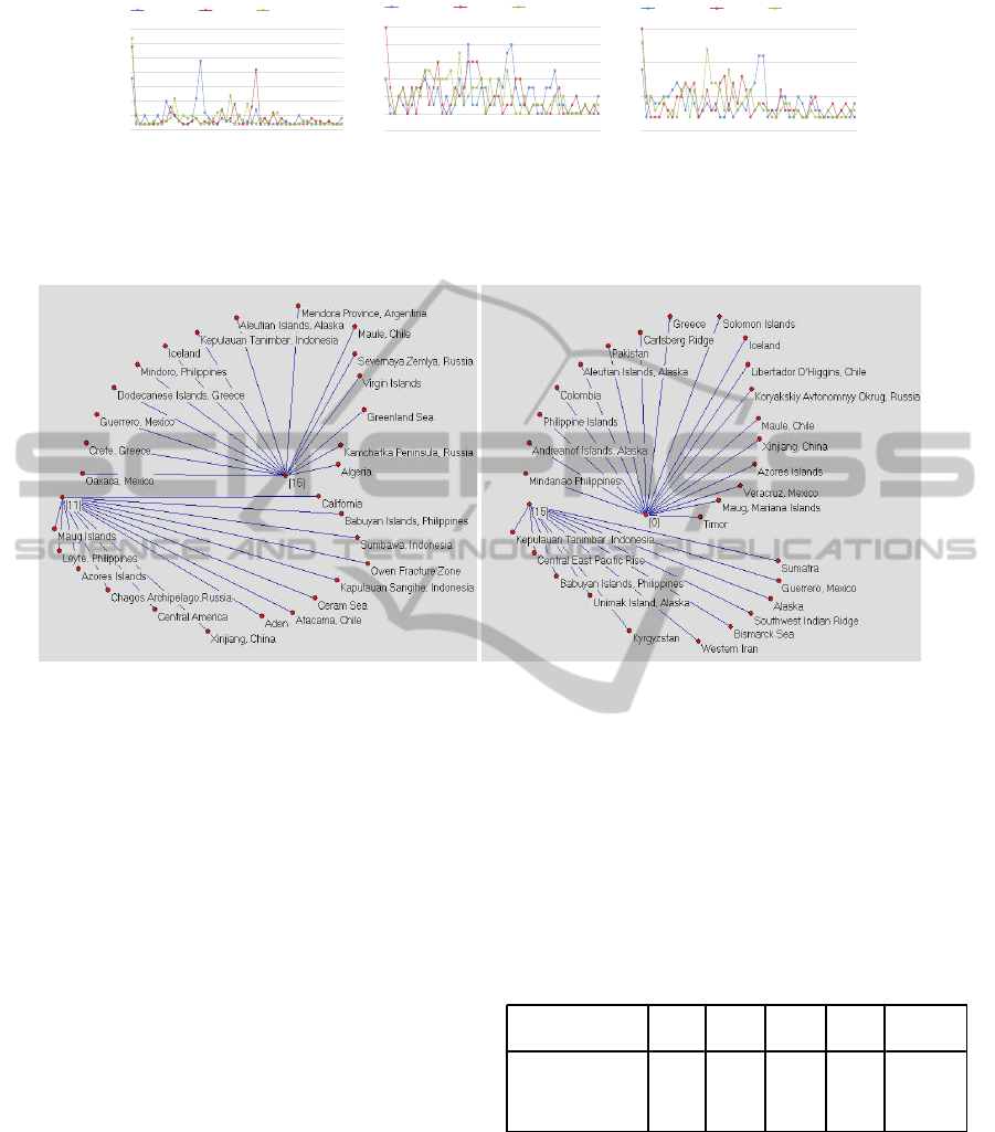
Figure 6: Place membership distribution in clusters for the Markov chain model, shown for the agglomerative single, complete,
and average linkage methods, and parameterized for each by year-week, monthly and bi-monthly resampling modes.
(a) Mixture model. (b) Markov chain.
Figure 7: Graphically visualized two cluster networks for each the mixture model and Markov chain clustering frameworks.
The Markov chain approach stands out in both find-
ing seismic relations for at least a pair of places, and
moreover, it employs the full set of fifty groups.
Figure 6 further depicts an interpretation of place
membership distribution for the Markov chain model,
reviewing the single, complete and average linking
methods, each parametrized by the seismic signal re-
sampling modes, including year-week, monthly and
bi-monthly intervals. Results pertaining to the Ward
linkage method are intentionally precluded to avoid
reporting any bias towards even place divisions. Par-
tition allocations for the complete and average link
functions appear on a fairly equal scale and show a
convincing behavior resemblance. Whereas at first
inspection, the simple similarity method differs strik-
ingly from the rest and has three peaks that stand
apart for groups of about 20 to 30 place members.
However, in barring the outliers and rescaling the re-
maining member counts, a clear indication of equiv-
alence ensues. While the place term frequency in a
cluster varies orthogonally to any of modifying the
linkage method or the resampling mode, notably is
the strong inclusive correlation often observed across
classes generated out-of-order by different linkage
methods. Figure 7(b) shows for network node 0 a su-
per group created by the single linkage, and Figure
8 presents for that node, both the complete and aver-
age similarity methods, producing subgroups that are
fully contained in the aforementioned super class.
Table 6: Statistical measures of distributed, cluster place
membership for the three clustering paradigms. The 1-Place
column identifies single member groups of no relations.
Model Min Max Med SD 1-Place
Flinn-Engdahl 0 24 2 4.48 8
Mixture Model 0 16 3 4.06 4
Markov Chain 2 24 3 4.07 0
Apart from the intuition of seismic similarity re-
sulting from geo-spatial proximity, as prescribed in
the Flinn-Engdahlmodel, we are interested in patterns
that relates places by their closeness in feature space,
for both the scale frequency and time series represen-
tations that feed into our mixture model and Markov
chain, respectively. Figure 7 shows graphically the
networks of two cluster nodes and their contextual
place descendants, for each of our clustering frame-
InferringGeo-spatialNeutralSimilarityfromEarthquakeDatausingMixtureandStateClusteringModels
13
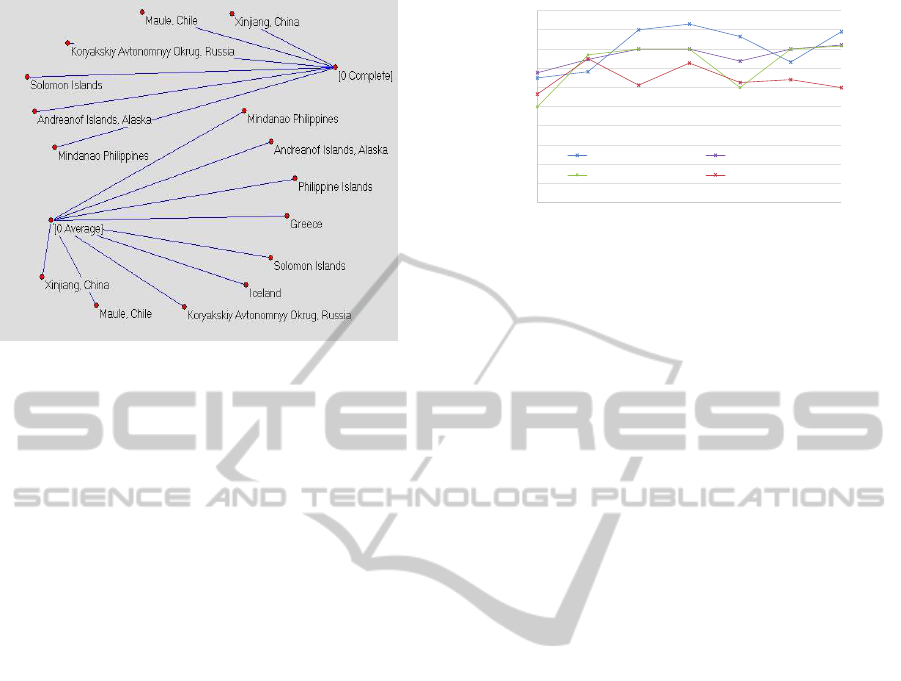
Figure 8: Graphically visualized cluster networks produced
by using complete and average linkage methods.
works. Emanating from a statistical process of group-
ing unlabeled earthquake bound locations, an imme-
diate observation of the cluster content identifies seis-
mic behavior similarities in geographical places that
are both close and far apart physically. For example,
cluster id 15 (Figure 7(a)), originated in the composi-
tion of scale distribution features, incorporates Euro-
pean, African, North and South American, and Asian
countries including Iceland, Greece, Algeria, Alaska,
Mexico, and the Philippines. Similarly, cluster id
11 (Figure 7(a)) has California from North America,
Aden in Africa, Eastern Europe Russia, and Asian In-
donesia. Corollary, assemblies of time series features
(Figure 7(b)) configure sites of different continents
and show little resemblance to the Flinn-Engdahl geo-
spatial regional scheme. The discovery of unsolicited
seismic patterns promotes less dependence on a con-
straint physical partition profile and encourages more
flexible and autonomous ecological relations, based
on objective macroseismic effects (Hough, 2014).
Our software is flexible to let the user set both
the number of quake affected places and the number
of clusters to generate, in each of the mixture model
and Markov chain formulations. Constructing groups
composed of a larger site count, enable us to perform
classification and measure system level accuracy. For
classification, we use a k-nearest neighbor (KNN)
(Cormen et al., 1990) baseline model that computes
a Euclidean-squared distance between a randomly se-
lected, test seismic vector against the remaining train-
ing feature vectors, in either a distribution scale or a
signal based representation. We then apply a normal-
ized majority rule to ten nearest samples to a test fea-
ture vector, and derive a seismic score. This score
is further accumulated and averaged for each cluster,
and the matching cluster corresponds to the highest
0
0.1
0.2
0.3
0.4
0.5
0.6
0.7
0.8
0.9
1
50 75 100 125 150 175 200
Maximum Accuracy
Places
Scale Distribution Signal, Year-Week
Signal, Monthly Signal, Bi-Monthly
Figure 9: Classification maximum accuracy as a function
of ascending number of places, split into five clusters and
parametrized by seismic feature type.
average scoring, cluster id. Figure 9 shows classifi-
cation maximum accuracy for a five-cluster partition
as a function of a non descending place count, and
parametrized by a seismic feature type. Scale distri-
bution features depict a slightly higher accuracy com-
pared to the seismic signal form, mostly ascribed to
sparseness of the latter due to samples of no seismic
action, and evidently, a coarser mode of time series
resampling results in a mild decline of accuracy rate.
To the best of our knowledge and based on lit-
erature published to date, we are unaware of seis-
mic analysis systems with similar goals to even-
handedly contrast our results against. The seismo-
surfer (Theodoridis, 2001), developed for seismic
data management and mining employs the k-means
algorithm for clustering. By specifying n geo-places
and k clusters, k-means time complexity is O (kn)
for each iteration, however the number of itera-
tions to converge can be very large. Conversely, in
our experiments both the EM and BW algorithms
ran efficiently well under 100 iterations to conver-
gence, along with setting the likelihood delta thresh-
old to 1e
−10
. Whereas computational complexity of
a bottom-up hierarchical clustering is O(n
2
logn), yet
the process terminates early once the desired num-
ber of clusters is reached. Another key architectural
difference is the localized spatio-temporal nature of
queries into the seismo-surfer database, as our design
seeks more broader shake relations that span the uni-
verse mostly unconditionally.
5 CONCLUSIONS
We have demonstrated the apparent potential in de-
ploying information retrieval and unsupervised ma-
chine learning methods, to accomplish the discov-
ery of geo-spatial free similarity of earthquake bound
places. By disregarding any prior location knowledge
GISTAM2015-1stInternationalConferenceonGeographicalInformationSystemsTheory,ApplicationsandManagement
14

from presumed unlabeled seismic data, our proposed
system is generic and scalable and relies entirely on
objective closeness metrics in feature space that re-
moves dependency on a more constraining regional
scheme. For each of our distribution and signal type
feature vectors, both cluster analysis and classifica-
tion results affirm seismic pattern relations that cross
continent boundaries, suggesting similarity of impar-
tial macroseismic effects.
The data we acquired comprised of a large number
of hundreds of thousands earthquake events, recorded
in an extended period of time of four decades, and af-
fected a few thousands sites around the world. How-
ever, only a few hundreds of places, each bearing at
least several hundreds of shake occurrences, are sta-
tistically reasoned and pertinent to our probabilistic
system approach. Advancing the growth of the seis-
mic training set is imperative to our work and directly
affects classification robustness. Yet using geograph-
ical locations that endured under one hundred seismic
events is a suboptimal choice for our system, giving
rise to highly sparse feature vectors. Alternatively, we
contend that by coalescing locations of a small event
count into a macro seismic site, based on geo-spatial
proximity considerations, our training collection size
is likely to increase further and proportionally let us
gain a more stable classification process.
A direct progression of our work is to assume
no foregoing knowledge of the number of seismic
clusters to generate, and discover both the model fit-
ting and the selection dimension directly from the in-
complete seismic training set, using a combination of
Akaike and Bayesian information criteria. We look
forward to further incorporate the three dimensional
geometrical data provided in a GeoJSON object, and
possibly detect seismic similarity along either a longi-
tude or a latitude extent perspective. Lastly, the flex-
ibility of our software allows us to pursue a higher
level, inter-cluster network study to better understand
second order set of seismic relations.
ACKNOWLEDGEMENTS
We would like to thank the anonymous reviewers for
their insightful and helpful feedback.
REFERENCES
Akaike, H. (1973). Information theory and an extension of
the maximum likelihood principle. In International
Symposium on Information Theory, pages 267–281,
Budapest, Hungary.
Baeza-Yates, R. and Ribeiro-Neto, B., editors (1999). Mod-
ern Information Retrieval. ACM Press Series/Addison
Wesley, Essex, UK.
Baum, L. E. (1972). An inequality and associated maxi-
mization technique in statistical estimation for proba-
bilistic functions of Markov processes. In Symposium
on Inequalities, pages 1–8, Los Angeles, CA.
Baum, L. E. and Petrie, T. (1966). Statistical inference for
probabilistic functions of finite state Markov chains.
Annals of Mathematical Statistics, 37(6):1554–1563.
Cormen, T. H., Leiserson, C. H., Rivest, R. L., and
Stein, C. (1990). Introduction to Algorithms. MIT
Press/McGraw-Hill Book Company, Cambridge, MA.
Dempster, A. P., Laird, N. M., and Rubin, D. B. (1977).
Maximum likelihood from incomplete data via the
EM algorithm. Royal Statistical Society, 39(1):1–38.
Duda, R. O., Hart, P. E., and Stork, D. G. (2001). Unsu-
pervised learning and clustering. In Pattern Classifi-
cation, pages 517–601. Wiley, New York, NY.
Flinn-Engdahl (2000). Flinn-Engdahl seismic and geo-
graphic regionalization scheme. http://earthquake.
usgs.gov/learn/topics/flinn
engdahl.php.
Fraley, C. and Raftery, A. E. (2002). Model-based
clustering, discriminant analysis and density estima-
tion. Journal of the American Statistical Association,
97(458):611–631.
Fraley, C. and Raftery, A. E. (2007). Bayesian regulariza-
tion for normal mixture estimation and model-based
clustering. Journal of Classification, 24(2):155–181.
GeoJSON (2007). Geojson format for encoding geographic
data structures. http://geojson.org/.
Hough, S. E. (2014). Earthquake intensity distribution:
A new view. Bulletin of Earthquake Engineering,
12(1):135–155.
Johnson, S. C. (1967). Hierarchical clustering schemes.
Psychometrika, 32(3):241–254.
Kaufman, L. and Rousseeuw, P. J., editors (1990). Finding
Groups in Data: An Introduction to Cluster Analysis.
Wiley, New York, NY.
Langfelder, P., Zhang, B., and Horvath, S. (2007). Defining
clusters from a hierarchical cluster tree: the dynamic
tree cut library for R. Bioinformatics, 24(5):719–720.
Manning, C. D., Raghavan, P., and Schutze, H. (2008). In-
troduction to Information Retrieval. Cambridge Uni-
versity Press, Cambridge, United Kingdom.
Manning, C. D. and Schutze, H., editors (2000). Founda-
tions of Statistical Natural Language Processing. MIT
Press, Cambridge, UK.
Mclachlan, G. J. and Basford, K. E. (1988). Mixture Mod-
els: Inference and Applications to Clustering. Marcel
Dekker, New York, NY.
Mclachlan, G. J. and Peel, D. (2000). Finite Mixture Mod-
els. John Wiley and Sons, New York, NY.
Ngatchou-Wandji, J. and Bulla, J. (2013). On choosing a
mixture model for clustering. Journal of Data Sci-
ence, 11(1):157–179.
R (1997). R project for statistical computing. http://
www.r-project.org/.
InferringGeo-spatialNeutralSimilarityfromEarthquakeDatausingMixtureandStateClusteringModels
15

Rabiner, L. R. (1989). A tutorial on hidden Markov models
and selected applications in speech recognition. Pro-
ceedings of IEEE, 77(2):257–286.
Rajaraman, R. and Ullman, J. D. (2011). Mining of Massive
Datasets. Cambridge University Press, New York,
NY.
Salton, G., Wong, A., and Yang, C. S. (1975). A vector
space model for automatic indexing. Communications
of the ACM, 18(11):613–620.
Schwarz, G. (1978). Estimating the dimension of a model.
The Annals of Statistics, 6(2):461–464.
Theodoridis, Y. (2001). SEISMO-SURFER: A prototype
for collecting, querying, and mining seismic data.
In Advances in Informatics, pages 159–171, Nicosia,
Cyprus.
USGS (2004). Real time feeds and notifications. http://
earthquake.usgs.gov/earthquakes/feed/v1.0/.
Ward, J. H. (1963). Hierarchical grouping to optimize an
objective function. American Statistical Association,
58(301):236–244.
Young, J. B., Presgrave, B. W., Aichele, H., Wiens, D. A.,
and Flinn, E. A. (1995). The Flinn-Engdahl region-
alization scheme: the 1995 revision. Physics of the
Earth and Planetary Interiors, 96(4):223–297.
GISTAM2015-1stInternationalConferenceonGeographicalInformationSystemsTheory,ApplicationsandManagement
16
