TIDAQL

A Query Language Enabling on-Line Analytical Processing of Time Interval Data

Philipp Meisen

, Diane Keng

, Tobias Meisen

, Marco Recchioni

and Sabina Jeschke

Institute of Information Management in Mechanical Engineering, RWTH Aachen University, Aachen, Germany

School of Engineering, Santa Clara University, Santa Clara, U.S.A.

Airport Devision, Inform GmbH Aachen, Aachen, Germany

Keywords: Time Interval Data, Query Language, on-Line Analytical Processing, Distributed Query Processing.

Abstract: Nowadays, time interval data is ubiquitous. The requirement of analyzing such data using known techniques

like on-line analytical processing arises more and more frequently. Nevertheless, the usage of approved mul-

tidimensional models and established systems is not sufficient, because of modeling, querying and processing

limitations. Even though recent research and requests from various types of industry indicate that the handling

and analyzing of time interval data is an important task, a definition of a query language to enable on-line

analytical processing and a suitable implementation are, to the best of our knowledge, neither introduced nor

realized. In this paper, we present a query language based on requirements stated by business analysts from

different domains that enables the analysis of time interval data in an on-line analytical manner. In addition,

we introduce our query processing, established using a bitmap-based implementation. Finally, we present a

performance analysis and discuss the language, the processing as well as the results critically.

1 INTRODUCTION

Nowadays, time interval data is recorded, collected

and generated in various situations and different ar-

eas. Some examples are the resource utilization in

production environments, deployment of personnel in

service sectors, or courses of diseases in healthcare.

Thereby, time interval data is used to represent obser-

vations, utilizations or measures over a period of

time. Put in simple terms, time interval data is defined

by two time values (i.e. start and end), as well as de-

scriptive values associated to the interval: like labels,

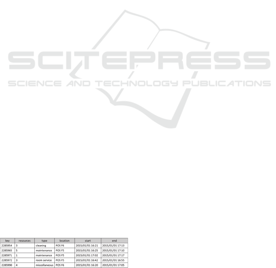
numbers, or more complex data structures. Figure 1

illustrates a sample database of five records.

Figure 1: A sample time interval database with intervals de-

fined by [start, end), an id, and three descriptive values.

For several years, business intelligence and ana-

lytical tools have been used by managers and business

analysts, inter alia, for data-driven decision support

on a tactical and strategic level. An important tech-

nology used within this field, is on-line analytical pro-

cessing (OLAP). OLAP enables the user to interact

with the stored data by querying for answers. This is

achieved by selecting dimensions, applying different

operations to selections (e.g. roll-up, drill-down, or

drill-across), or comparing results. The heart of every

OLAP system is a multidimensional data model

(MDM), which defines the different dimensions, hi-

erarchies, levels, and members (Codd, 1993).

The need of handling and analyzing time interval

data using established, reliable, and proven technolo-

gies like OLAP is desirable in this respect and an es-

sential acceptance factor. Nevertheless, the MDM

needed to model time interval data has to be based on

many-to-many relationships which have been shown

to lead to summarizability problems. Several solu-

tions solving these problems on different modeling

levels have been introduced over the last years, lead-

ing to increased integration effort, enormous storage

needs, almost always inacceptable query perfor-

mances, memory issues, and often complex multidi-

mensional expressions (Mazón et al., 2008; Kimball

and Rose, 2013). Additionally, these solutions are,

Meisen P., Keng D., Meisen T., Recchioni M. and Jeschke S..

TIDAQL - A Query Language Enabling on-Line Analytical Processing of Time Interval Data.

DOI: 10.5220/0005348400540066

In Proceedings of the 17th International Conference on Enterprise Information Systems (ICEIS-2015), pages 54-66

ISBN: 978-989-758-096-3

 2015 SCITEPRESS (Science and Technology Publications, Lda.)

considering real-world scenarios, only applicable to

many-to-many relationships having a small cardinal-

ity which is mostly not the case when dealing with

time interval data. As a result, the usage of MDM and

available OLAP systems is not sufficient, even

though the operations (e.g. roll-up, drill-down, slice,

or dice) available through such systems are desired.

Enabling such OLAP like operations in the con-

text of time interval data, requires the provision of ex-

tended filtering and grouping capabilities. The former

is achieved by matching descriptive values against

known filter criteria logically connected using opera-

tors like and, or, or not, as well as a support of tem-

poral relations like starts-with, during, overlapping,

or within (Allen, 1983). The latter is applied by

known aggregation operators like max, min, sum, or

count, as well as temporal aggregation operators like

count started or count finished (Meisen et al., 2015).

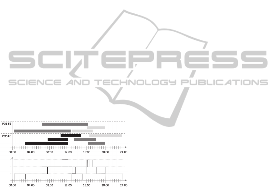
The application of the count aggregation operator

for time interval data is exemplified in Figure 2. The

color code identifies the different types of a time in-

terval (e.g. cleaning, maintenance, room service, mis-

cellaneous). Furthermore, the swim-lanes show the

location. The figure illustrates the count of intervals

for each type over one day across all locations (e.g.

POS F5 and POS F6) using a granularity of minutes

(i.e. 1,440 aggregations are calculated).

Figure 2: On top the time interval data (10 records) shown

in a Gantt-Chart, on the bottom the aggregated time-series.

In this paper, we present a query language allow-

ing to analyze time interval data in an OLAP manner.

Our query language includes a data definition (DDL),

a data control (DCL), and a data manipulation lan-

guage (DML). The former is based on the time inter-

val data model introduced by Meisen et al., (2014),

whereby the latter supports the two-step aggregation

technique mentioned in Meisen et al., (2015). Fur-

thermore, we outline our query processing which is

based on a bitmap-based implementation and sup-

ports distributed computing.

This paper is organized as follows: In section 2,

we discuss related work done in the field of time in-

terval data, in particular this section provides a conci-

se overview of research dealing with the analyses of

time interval data. We provide an overview of time

interval models, discuss related work done in the field

of OLAP, and present query languages. In section 3,

we introduce our query language and processing. The

section presents among other things how a model is

defined and loaded, how temporal operators are ap-

plied, how the two-step aggregation is supported, how

groups are defined, and how filters are used. We in-

troduce implementation issues and empirically evalu-

ate the performance regarding the query processing in

section 4. We conclude with a summary and direc-

tions for future work in section 5.

2 RELATED WORK

When defining a query language, it is important to

have an underlying model, defining the foundation

for the language (e.g. the relational model for SQL,

different interval-based models for e.g. IXSQL or

TSQL2, the multidimensional model for MDX, or the

graph model for Cypher). Over the last years several

models have been introduced in the field of time in-

tervals, e.g. for temporal databases (Böhlen et al.,

1998), sequential pattern mining (Papapetrou et al.,

2009, Mörchen, 2009), association rule mining

(Höppner and Klawonn, 2001), or matching

(Kotsifakos et al., 2013).

Chen et al., (2003) introduced the problem of min-

ing time interval sequential patterns. The defined

model is based on events used to derive time inter-

vals, whereby a time interval is determined by the

time between two successive time-points of events.

The definition is based on the sequential pattern min-

ing problem introduced by Agrawal and Srikant

(1995). The model does not include any dimensional

definitions, nor does it address the labeling of time

intervals with descriptive values.

Papapetrou et al., (2005) presented a solution for

the problem of “discovering frequent arrangements of

temporal intervals”. An e-sequence is an ordered set

of events. An event is defined by a start value, an end

value and a label. Additionally, an e-sequence data-

base is defined as a set of e-sequences. The definition

of an event given by Papapetrou et al., is close to the

underlying definition within this paper (cf. Figure 1).

Nevertheless, facts, descriptive values, and dimen-

sions are not considered.

Mörchen (2006) introduced the TSKR model de-

fining tones, chords, and phrases for time intervals.

Roughly speaking, the tones represent the duration of

intervals, the chords the temporal coincidence of

tones, and the phrases represent the partial order of

TIDAQL-AQueryLanguageEnablingon-LineAnalyticalProcessingofTimeIntervalData

chords. The main purpose of the model presented by

Mörchen is to overcome limitations of Allen’s (1983)

temporal model considering robustness and ambigu-

ousness when performing sequential pattern mining.

The model neither defines dimensions, considers

multiple labels, nor recognizes facts.

Summarized, models presented in the field of se-

quential pattern mining, association rule mining or

matching do generally not define dimensions and are

focused on generalized interval data, or support only

non-labelled data. Thus, these models are not suitable

considering OLAP of time interval data, but are a

guidance to the right direction.

Within the research community of temporal data-

bases different interval-based models have been de-

fined (cf. Böhlen et al., 1998). The provided defini-

tions can be categorized in weak and strong models.

A weak model is one, in which the intervals are used

to group time-points, whereas the intervals of the lat-

ter carry semantic meaning. Thus, a weak interval-

based model is not of further interest from an analyt-

ical point of view, because it can be easily trans-

formed into a point-based model. Nevertheless, a

strong model and the involved meaning of the differ-

ent operators – especially aggregation operators – are

of high interest from an analytical view. Strong inter-

val-based models presented in the field of temporal

databases lack to define dimensions, but present im-

portant preliminary work.

In the field of OLAP, several systems capable of

analyzing sequences of data have been introduced

over the last years. Chui et al. (2010) introduced S-

OLAP for analyzing sequence data. Liu and Runden-

steiner (2011) analyzed event sequences using hierar-

chical patterns, enabling OLAP on data streams of

time point events. Bebel et al., (2012) presented an

OLAP like system enabling time point-based sequen-

tial data to be analyzed. Nevertheless, the system nei-

ther support time intervals, nor temporal operators.

Recently, Koncilia et al., (2014) presented I-OLAP,

an OLAP system to analyze interval data. They claim

to be the first proposing a model for processing inter-

val data. The definition is based on the interval defi-

nition of Chen et al., (2003) which defines the inter-

vals as the gap between sequential events. However,

Koncilia et al., assume that the intervals of a specific

event-type (e.g. temperature) for a set of specific de-

scriptive values (e.g. POS G2) are non-overlapping

and consecutive. Considering the sample data shown

in Figure 1, the assumption of non-overlapping inter-

vals is not valid in general (cf. record 2,285,965 and

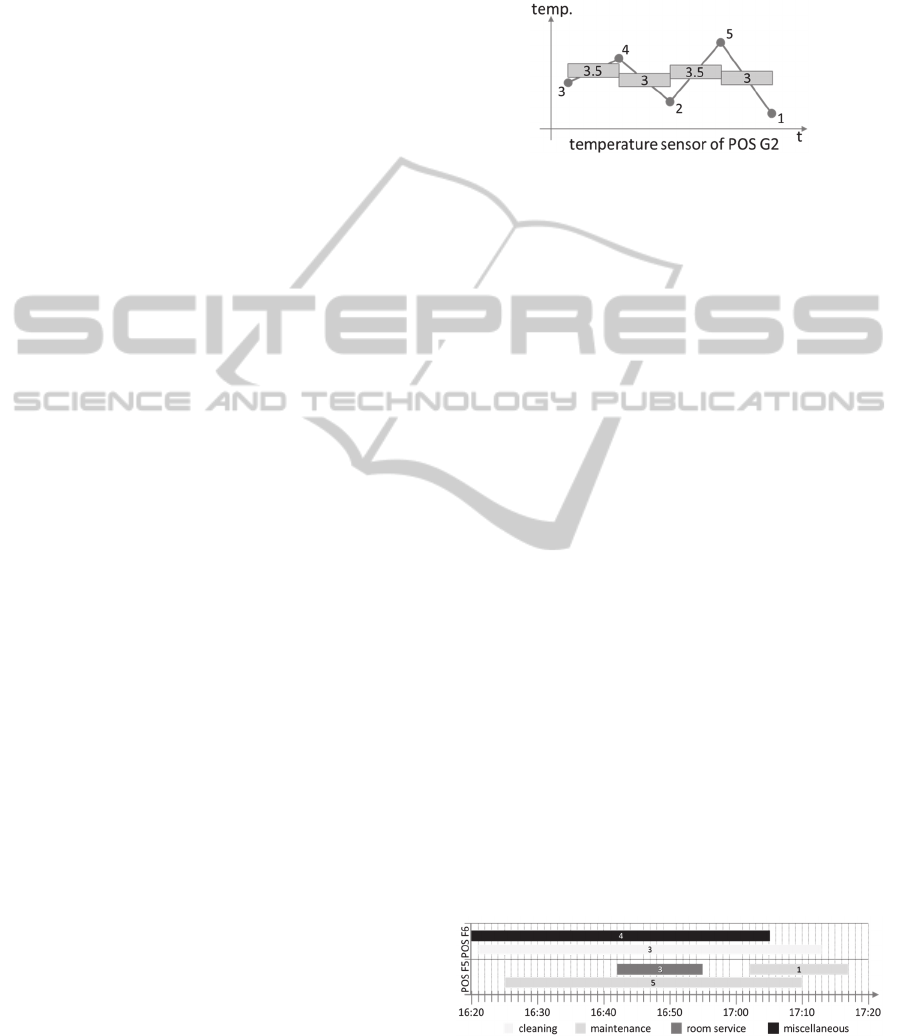
2,285,971). Figure 3 illustrates the model of Koncilia

et al. showing five temperature events for POS G2

and the intervals determined for the events. Koncillia

et al. mention the support of dimensions, hierarchies,

levels, and members, but lack to specify what types

of hierarchies are supported and how e.g. non-strict

relations are handled.

Figure 3: Illustration of the model introduced by Koncilia

et al., (2014). The intervals (rectangles) are created for each

two consecutive events (dots). The facts are calculated us-

ing the average function as the compute value function.

Also recently, Meisen et al., (2014) introduced the

IDA

ODEL

“enabling the usage of time interval data

for data-driven decision support”. The presented

model is defined by a 5-tuple ,,,, in which

 denotes the time interval database,  the set of de-

scriptors,  the time axis,  the set of measures, and

 the set of dimensions. The time interval database 

contains the raw time interval data records and a

schema definition of the contained data. The schema

associates each field of the record (which might con-

tain complex data structures) to one of the following

categories: temporal, descriptive, or bulk. Each de-

scriptor of the set  is defined by its values (more spe-

cific its value type), a mapping- and a fact-function.

The mapping-function is used to map the descriptive

values of the raw record to one or multiple descriptor

values. The mapping to multiple descriptor values al-

lows the definition of non-strict fact-dimension rela-

tionships. Additionally, the model defines the time

axis to be finite and discrete, i.e. it has a start, an end,

and a specified granularity (e.g. minutes). The set of

dimensions  can contain a time dimension (using a

rooted plane tree for the definition of each hierarchy)

and a dimension for each descriptor (using a directed

acyclic graph for a hierarchy’s definition). Figure 4

illustrates the modeled sample database of Figure 1

using the T

IDA

ODEL

Figure 4: Data of the sample database shown in Figure 1

modeled using the T

IDA

ODEL

(Meisen et al., 2014).

The figure shows the five intervals, as well as the

ICEIS2015-17thInternationalConferenceonEnterpriseInformationSystems

values of the descriptors location (cf. swim-lane) and

type (cf. legend). Dimensions are not shown. The

used mapping function for all descriptors is the iden-

tity function. The used granularity for the time dimen-

sion is minutes.

Another important aspect when dealing with time

interval data in the context of OLAP, is the aggrega-

tion of data and the provision of temporal aggregation

operators. Kline and Snodgrass (1995) introduced

temporal aggregates, for which several enhanced al-

gorithms were presented over the past years. Never-

theless, the solutions are focused on one specific ag-

gregation operator (e.g. SUM), do not support multi-

ple filter criteria, or do not consider data gaps. Kon-

cilia et al., (2014) address shortly how aggregations

are performed using the introduced compute value

functions and fact creating functions. Temporal oper-

ators are neither defined nor mentioned. Koncilia et

al., point out that some queries need special attention

when aggregating the values along time, but a more

precise problem statement is not given. Meisen et al.,

(2015) introduce a two-step aggregation technique for

time interval data. The first one aggregates the facts

along the intervals of a time granule and the second

one aggregates the values of the first step depending

on the selected hierarchy level of the time dimension.

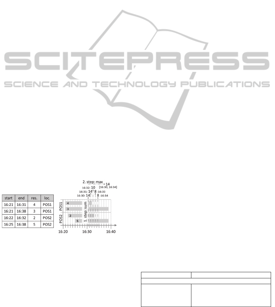
Figure 5 illustrates the two-step aggregation tech-

nique. In the illustration, the technique is used to de-

termine the needed resources within the interval

[16:30, 16:34]. Within the first step, the sum of the

resources for each granule is determined and within

the second step the maximum of the determined val-

ues is calculated, i.e. 14. Additionally, they introduce

temporal aggregation operators like started or fin-

ished count.

Figure 5: Two-step aggregation technique presented by

Meisen et al., (2015).

The definition of a query language based on a

model and operators (i.e. like aggregations), is com-

mon practice. Regarding time-series, multiple query

languages and enhancements of those have been in-

troduced (cf. Rafiei and Mendelzon, 2000). In the

field of temporal databases time interval-based query

languages like IXSQL, TSQL2, or ATSQL have been

defined (Böhlen et al., 1998) and within the analytical

field, MDX (Spofford et al., 2006) is a widely used

language to query MDMs. Considering models deal-

ing with time interval data in the context of analytics,

Koncilia et al., (2014) published the only work the

authors are aware of that mentions a query language.

Nevertheless, the query language is neither formally

defined nor further introduced.

Summarized, it can be stated that recent research

and requests from industry indicate that the handling

of time interval data in an analytical context is an im-

portant task. Thus, a query language is required capa-

ble of covering the arising requirements. Koncilia et

al., (2014) and Meisen et al., (2014, 2015) introduced

two different models useful for OLAP of time interval

data. Different temporal aggregation operators, as

well as standard aggregation operators, are also pre-

sented by Meisen (2015). Nevertheless, a definition

of a query language useful for OLAP and an imple-

mentation of the processing are, to the best of our

knowledge, not formally introduced.

3 THE TIDA QUERY LANGUAGE

In this section, we introduce our time interval data

analysis query language (T

IDA

QL). The language was

designed for a specific purpose; to query time interval

data from an analytical point of view. The language

is based on aspects of the previously discussed

IDA

ODEL

. Nevertheless, the language should be

applicable to any time interval database system which

is capable of analyzing time interval data. Neverthe-

less, some adaptions might be necessary or some fea-

tures might not be supported by any system.

3.1 Requirements

The requirements concerning the query language and

its processing were specified during several work-

shops with over 70 international business analysts

from different domains (i.e. aviation industry, logis-

tics providers, service providers, as well as language

and gesture research). We aligned the results of the

workshop with an extended literature research. Table

1 summarizes selected results.

Table 1: Summary of the requirements concerning the time

interval analysis query language (selected results).

Requirement Description

Data Control Language (DCL)

[DCL1]: authorization

aspects

It is expected that the language encom-

passes authorization features, e.g. user

deletion, role creation, granting and re-

voking permissions.

TIDAQL-AQueryLanguageEnablingon-LineAnalyticalProcessingofTimeIntervalData

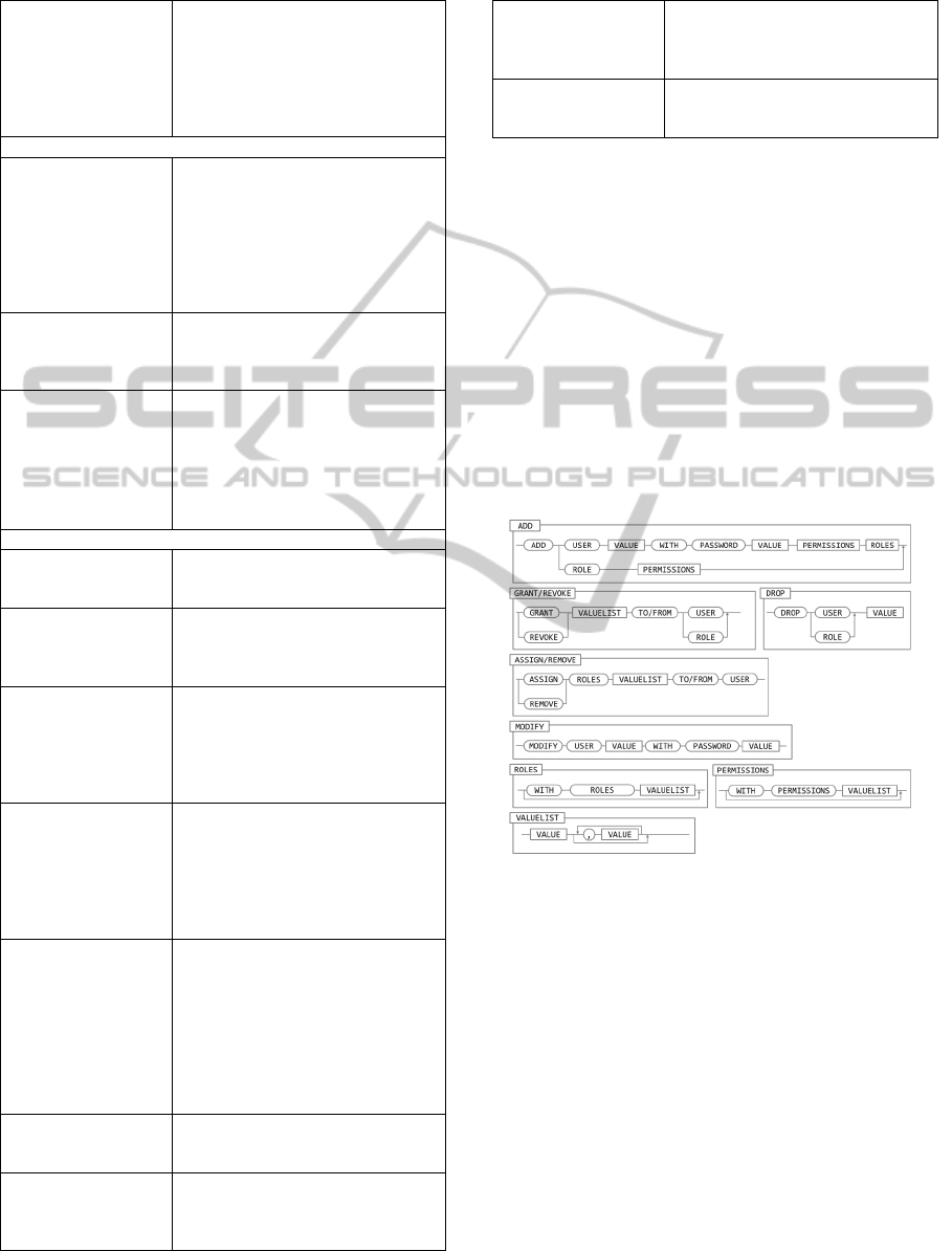
Table 1: Summary of the requirements concerning the time

interval analysis query language (selected results). (cont.)

[DCL2]: permissions

grantable on global and

model level

Permissions must be grantable on a

model and a global level. It is expected

that the user can have the permission to

add data to one model but not to an-

other. For simplicity, it should be pos-

sible to grant or revoke several permis-

sions at once.

Data Definition Language (DDL)

[DDL1]: loading and

unloading

The language has to offer a construct to

load new and unload models. The

newly loaded model has to be available

without any restart of the system. An

unloaded model has to be unavailable

after the query is processed. However,

queries currently in process must still

be executed.

[DDL2]: non-onto,

non-covering, non-

strict hierarchies

Each descriptor dimension must sup-

port hierarchies which might be non-

onto, non-covering, and / or non-strict

(cf. Pedersen, 2000).

[DDL3]: raster levels A raster level is a level of the time di-

mension. For example: the 5-minute

raster-level defines members like

[00:00, 00:05) … [23:55, 00:00). Sev-

eral raster levels can form a hierarchy

(e.g. 5-min  30-min  60-min 

half-day  day).

Data Manipulation Language (DML)

[DML1]: raw data

records

The language must provide a construct

to select the raw time interval data rec-

ords.

[DML2]: time-series by

time-windows

The language must support the specifi-

cation of a time-window for which

time-series of different measures can be

retrieved.

[DML3]: temporal

operators

It must be possible to use temporal op-

erators for filtering as e.g. defined by

Allen (1983). Depending on the type of

selection (i.e. raw records or time-se-

ries) the available temporal operators

may differ.

[DML4]: The two-step

aggregation technique

Meisen et al., (2015) present a two-step

aggregation technique which has to be

supported by the language. Both aggre-

gation operators (see Figure 5) must be

specified by a query selecting time-se-

ries, no pre-defined measure should be

necessary.

[DML5]: complete

time-series

A time-series is selected by specifying

a time-window (e.g. [01.01.2015,

02.01.2015) and a level (e.g. minutes).

The resulting time-series must contain

a value for each member of the selected

level, even if no time interval covers the

specified member. The value might be

N/A or null to indicate missing infor-

mation.

[DML6]: insert, update

and delete

The language must offer constructs to

insert, update and delete time interval

data records.

[DML7]: open, half-

open, or closed

intervals

The system should be capable of inter-

preting intervals defined as open, e.g.

(0, 5), closed, e.g. [0, 5], or half-

opened, e.g. (0, 5].

Table 1: Summary of the requirements concerning the time

interval analysis query language (selected results). (cont.)

[DML8]: meta-

information

It is desired that the language supports

a construct to receive meta-information

from the system, e.g. actual version,

available users, or loaded models.

[DML9]: bulk load It is desired, that the language provides

a construct to enable a type of bulk

load, i.e. increased insert performance.

3.2 Data Control Language

The definition of the DCL is straight forward to the

DCL known from other query languages e.g. SQL. As

defined by requirement [DCL1], the language must

encompass authorization features. Hence, the lan-

guage contains commands like ADD, DROP, MODIFY,

GRANT, REVOKE, ASSIGN and REMOVE. In our imple-

mentation, the execution of a DCL command always

issues a direct commit, i.e. a roll back is not sup-

ported. Figure 6 shows the syntax diagram of the

commands. Because of simplicity, a value is not fur-

ther specified and might be a permission, a username,

a password, or a role.

Figure 6: Commands of the DCL query language.

To fulfill the [DCL2] requirement, we define a

permission that consists of a scope-prefix and the per-

mission itself. We define two permission-scopes

GLOBAL and MODEL. Thus, a permission of the

GLOBAL scope is defined by

GLOBAL.<permission>

(e.g. GLOBAL.manageUser). Instead, a permission

of the MODEL scope is defined by

MODEL.<model>.<permission>

(e.g. MODEL.myModel.query).

For query processing, we use the Apache Shiro au-

thentication framework (http://shiro.apache.org/).

ICEIS2015-17thInternationalConferenceonEnterpriseInformationSystems

Shiro offers annotation driven access control. Thus,

the permission to e.g. execute a DML query is per-

formed by annotating the processing query method.

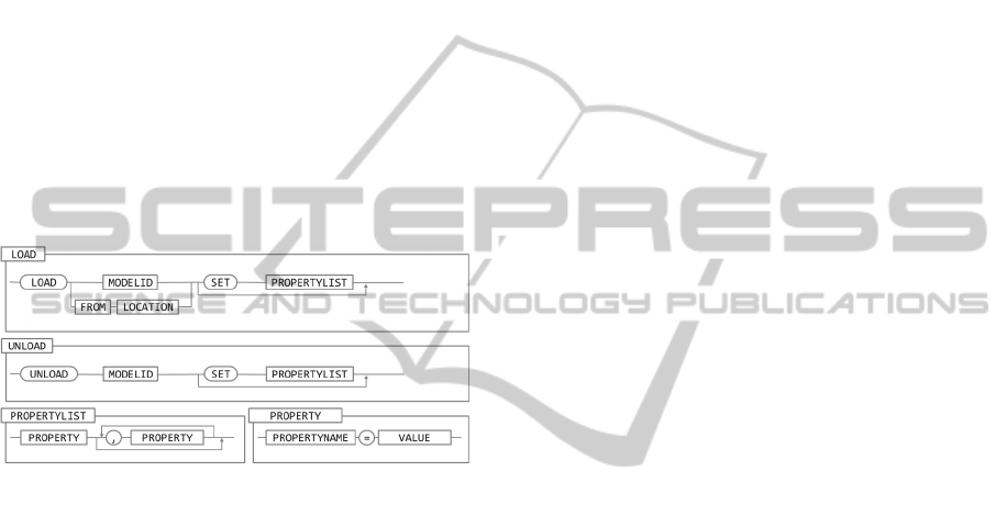
3.3 Data Definition Language

The DDL is used to define, add, or remove the models

known by the system. [DDL1] requires a command

within the DDL which enables the user to load or un-

load a model. The syntax diagram of the LOAD and

UNLOAD command is shown in Figure 7. A model can

be loaded by using a model identifier already known

to the system (e.g. if the model was unloaded), or by

specifying a location from which the system can re-

trieve a model definition to be loaded. Additionally,

properties can be defined (e.g. the autoload property

can be set, to automatically load a model when the

system is started). In the following subsection, we

present an XML used to define a T

IDA

ODEL

Figure 7: Commands of the DDL query language.

3.3.1 The XML T

IDA

ODEL

Definition

As mentioned in section 2, the T

IDA

ODEL

is defined

by a 5-tuple ,,,,. The time interval database

 contains the raw record inserted using the API or

the INSERT command introduced later in section

3.4.1. From a modelling perspective it is important for

the system to retrieve the descriptive and temporal

values from the raw record. Thus, it is essential to de-

fine the descriptors  and the time axis  within the

XML definition. Below, an excerpt of an XML file

defining the descriptors of our sample database

shown in Figure 1 is presented:

</descriptors>

</model>

The excerpts shows that a descriptor is defined by a

tag specifying the type (i.e. the descriptor implemen-

tation to be used), an id-attribute, and an optional

name-attribute. Additionally, it is possible to define if

the descriptor allows null values (default) or not. To

support more complex data structures (and one’s own

mapping functions), it is possible to specify one’s

own descriptor-implementations:

<ownImpl:list id="D4" />

</descriptors>

Our implementation scans the class-path automati-

cally, looking for descriptor implementations. An

added implementation must provide an XSLT file,

placed into the same package and named as the con-

crete implementation of the descriptor-class. The

XSLT file is used to create the instance of the own

implementation using a Spring Bean configuration

(http://spring.io/).

<xsl:template match="ownImpl:list">

<xsl:call-template name="beanDesc">

<xsl:with-param name="class">

my.own.desc.List

</xsl:with-param>

</xsl:call-template>

</xsl:template>

The time axis of the T

IDA

ODEL

is defined by:

<time>

<timeline start="20.01.1981"

end="20.01.2061"

granularity="MINUTE" />

</time>

</model>

The time axis may also be defined using integers, i.e.

[0, 1000]. Our implementation includes two default

mappers applicable to map different types of temporal

raw record value to a defined time axis. Nevertheless,

sometimes it is necessary to use different time-map-

pers (e.g. if the raw data contains proprietary tem-

poral values) which can be achieved using the same

mechanism as described previously for descriptors.

Due to the explicit time semantics, the measures

defined within the T

IDA

ODEL

are different than

the ones typically known from an OLAP definition.

The model defines three categories for measures, i.e.

implicit time measures, descriptor bound measures,

and complex measures. The categories determine

when which data is provided during the calculation

process of the measures. Our implementation offers

several aggregation operators useful to specify a

measure, i.e. count, average, min, max, sum, mean,

median, or mode. In addition, we implemented two

temporal aggregation operators started count and

finished count, as suggested by Meisen et al., (2015).

TIDAQL-AQueryLanguageEnablingon-LineAnalyticalProcessingofTimeIntervalData

We introduce the definition and usage of measures in

section 3.4.2.

The T

IDA

ODEL

also defines the set of dimen-

sions . The definition differs between descriptor di-

mensions and a time dimension, whereby every di-

mension consists of hierarchies, levels, and members.

It should be mentioned that, from a modelling point

of view, each descriptor dimension fulfills the re-

quirements formalized in [DDL2] and that the time

dimension supports raster-levels as requested in

[DDL3]. The definition of a dimension for a specific

descriptor or the time dimension can be placed within

the XML definition of a model using:

<member id="ADV" reg="TENT"

rollUp="*" />

</level>

<member id="POSF" reg="POS F\d"

rollUp="DREAM" />

<member id="POSG" reg="POS G\d"

rollUp="DREAM" />

</level>

<member id="POSA" reg="POS A\d"

rollUp="STAR" />

</level>

</hierarchy>

</dimension>

</dimensions>

</model>

Figure 8 illustrates the descriptor dimension defined

by the previously shown XML excerpt. The circled

nodes are leaves which are associated with descriptor

values known by the model (using regular expres-

sions). Additionally, it is possible to add dimensions

for analytical processes to an already defined model,

i.e. to use it only for a specific session or query. The

used mechanism to achieve that is similar to the load-

ing of a model and will not further be introduced.

Figure 8: Illustration of the dimension created with our

web-based dimension-modeler as defined by the XML ex-

cerpt.

The definition of a time dimension is straight for-

ward to the one of a descriptor dimension. Neverthe-

less, we added some features in order to ease the def-

inition. Thus, it is possible to define a hierarchy by

using pre-defined levels (e.g. templates like

5-min-raster, day, or year) and by defining the level

to roll up to, regarding the hierarchy. The following

XML excerpt exemplifies the definition:

<level id="YEAR" template="YEAR"

rollUp="*" />

<level id="DAY" template="DAY"

rollUp="YEAR" />

<level id="60R" template="60RASTER"

rollUp="DAY" />

<level id="5R" template="5RASTER"

rollUp="60R" />

<level id="LG" template="LOWGRAN"

rollUp="5R" />

</hierarchy>

</timedimension>

</dimensions>

</model>

A defined model is published to the server using the

LOAD command. The following subsection introduces

the command, focusing on the loading of a model

from a specified location.

3.3.2 Processing the LOAD Command

The loading of a model can be triggered from differ-

ent applications, drivers, or platforms. Thus, it is nec-

essary to support different loaders to resolve a speci-

fied location. In the following, some examples illus-

trate the issue. When firing a LOAD query from a web-

application, it is necessary that the model definition

was uploaded to the server, prior to executing the

query. While running on an application server, it

might be required to load the model from a database

instead of loading it from the file-system. Thus, we

added a resource-loader which can be specified for

each context of a query. Within a servlet, the loader

resolves the specified location against the upload-di-

rectory, whereby our JDBC driver implementation is

capable of sending a client’s file to the server using

the data stream of the active connection. After retriev-

ing and validating the resource, the implementation

uses a model-handler to bind and instantiate the de-

fined model. As already mentioned, the bitmap-based

implementation presented by Meisen et al., (2015) is

used. The implementation instantiates several indexes

and bitmaps for the defined model. After the

instantiation, the model is marked to be up and run-

ICEIS2015-17thInternationalConferenceonEnterpriseInformationSystems

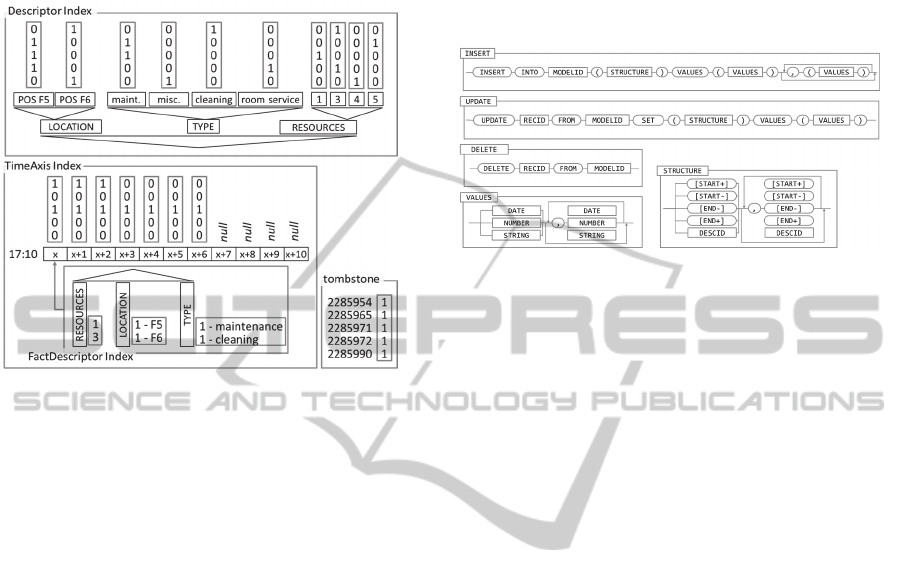
ning by the model-handler and accepts DML queries.

Figure 9 exemplifies the initialized bitmap-based in-

dexes filled with the data from the database of Figure

Figure 9: Example of a loaded model (cf. Meisen et al.,

2015) filled with the data shown in Figure 1.

3.4 Data Manipulation Language

Considering the requirements, it can be stated that the

DML must contain commands to INSERT, UPDATE,

and DELETE records. In addition, it is necessary to

provide SELECT commands to retrieve the time inter-

val data records, as well as results retrieved from ag-

gregation (i.e. time-series). Furthermore, a GET com-

mand to retrieve meta-information of the system is

needed.

3.4.1 INSERT,UPDATE and DELETE

Figure 10 illustrated the three commands INSERT,

UPDATE, and DELETE using syntax diagrams which

fulfill the requirement [DML6]. The INSERT com-

mand adds one or several time interval data records

to the system. First, it parses the structure of the data

to be inserted. The query-parser validates the correct-

ness of the structure, i.e. the structure must contain

exactly one field marked as start and exactly one field

marked as end even though the syntax diagram sug-

gest differently. Additionally, the parser verifies if a

descriptor (referred by its id) really exists within the

model. Finally, it reads the values and invokes the

processor by passing the structure, as well as the val-

ues. The processor iterates over the defined values,

validates those against the defined structure, uses the

mapping functions of the descriptors to receive the

descriptor values, and calls the mapping function of

the time-axis. The result is a so-called processed rec-

ord which is used to update the indexes. The persis-

tence layer of the implementation ensures that the raw

record and the indexes get persisted. Finally, the

tombstone bitmap is updated which ensures that the

data is available within the system.

Figure 10: Syntax diagrams of the commands INSERT,

UPDATE and DELETE.

A deletion is performed by setting the tombstone

bitmap for the specified id to 0. This indicates that the

data of the record is not valid and thus the data will

not be considered by any query processors anymore.

The internally scheduled clean-up process removes

the deleted records and releases the space.

An update is performed by deleting the record

with the specified identifier and inserting the record

as described above.

To support bulk load, as desired by [DML9], an

additional statement is introduced. The statement

SET BULK TRUE is used to enable the bulk load,

whereby SET BULK FALSE stops the bulk loading

process. When enabling the bulk load, the system

waits until all currently running INSERT, UPDATE, or

DELETE queries of other sessions are performed. New

queries of that type are rejected across all sessions

during the waiting and processing phase. When all

queries are handled, the system responds to the bulk-

enabling query and expects an insert-like statement,

whereby the system directly starts to parse the incom-

ing data stream. As soon as the structure is known, all

incoming values are inserted. The indexes are only

updated in memory. If and only if the memory capac-

ity reaches a specified threshold, the persistence-layer

is triggered. In this case, the current data in memory

is flushed and persisted using the configured persis-

tence-layer (e.g. using the file-system, a relational da-

tabase, or any other NoSQL database). The memory

is also flushed and persisted whenever a bulk load is

finished.

TIDAQL-AQueryLanguageEnablingon-LineAnalyticalProcessingofTimeIntervalData

3.4.2 SELECTRaw Records and

Time-series

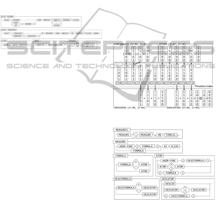
The SELECT command is addressed by the require-

ments [DML1], [DML2], [DML3], [DML4],

[DML5], and [DML7]. Figure 11 illustrates the select

statements to select records and time-series. Because

of space limitations, we removed more detailed syn-

tax diagrams for the LOGICAL and GROUP

EXPRESSION. The non-terminal MEASURES is speci-

fied later in this subsection when introducing the

SELECTTIMESERIES in detail.

Figure 11: Syntax diagrams of the SELECT RECORDS and

SELECTTIMESERIES commands.

As illustrated, the intervals can be defined as

open, half-open or closed (cf. [DML7]). The pro-

cessing of the intervals is possible, thanks to the dis-

crete time-axis used by the model. Using a discrete

time-axis with a specific granularity makes it easy to

determine the previous or following granule. Thus,

every half-open or open interval can be transformed

into a closed interval using the previous or following

granule. Hence, the result of the parsing always con-

tains a closed interval which is used during further

query processing.

As illustrated in Figure 11, the SELECTRECORDS

statement allows to retrieve records satisfying a logi-

cal expression based on descriptor values (e.g.

LOC="POS F5" OR (TYPE="cleaning" AND

DIMLOC.LOC.HOTEL="DREAM")) and/or fulfilling a

temporal relation (cf. [DML3]). Our query language

supports ten different temporal relations following

Allen (1983): EQUALTO, BEFORE, AFTER, MEETING,

DURING, CONTAINING, STARTINGWITH, FINISH‐

INGWITH, OVERLAPPING, and WITHIN. The inter-

ested reader may notice that Allen introduced thirteen

temporal relationships. We removed some inverse re-

lationships (i.e. inverse of meet, overlaps, starts, and

finishes). When using a temporal relationship within

a query, the user is capable of defining one of the in-

tervals used for comparison. Thus, the removed in-

verse relationships are not needed, instead the user

just modifies the self-defined interval. In addition, we

added the WITHIN relationship which is a combina-

tion of several relationships and allows an easy selec-

tion of all records within the user-defined interval (i.e.

at least one time-granule is contained within the user-

defined interval).

When processing a SELECT RECORD query, the

processor initially evaluates the filter expression and

retrieves a single bitmap specifying all records ful-

filling the filter’s logic (cf. Meisen et al., 2015). In a

second phase, the implementation determines a

bitmap of records satisfying the specified temporal re-

lationship. The two bitmaps are combined using the

and-operator to retrieve the resulting records. De-

pending on the requested information (i.e. count,

identifiers, or raw records (cf. [DML1])), the imple-

mentation creates the response using bitmap-based

operations (i.e. count and identifiers) or retrieving the

raw records from the persistence layer. Figure 12 de-

picts the evaluation of selected temporal relationships

using bitmaps and the database shown in Figure 1.

Figure 12: Examples of the processing of temporal relation-

ships using bitmaps (and the sample database of Figure 1).

Figure 13: Syntax diagrams of the MEASURES definition.

The SELECTTIMESERIES statement specifies a

logical expression equal to the one exemplified in the

SELECT RECORDS statement. In addition, the state-

ment specifies a GROUP EXPRESSION which de-

fines the groups to create the time-series for (e.g.

ICEIS2015-17thInternationalConferenceonEnterpriseInformationSystems

GROUPBYDIMLOC.LOC.ROOMS). Furthermore, the

measures to be calculated for the time-series and the

time-window (cf. [DML2]) are specified. It is also

possible to specify several comma-separated mea-

sures. Figure 13 shows the syntax used to specify

measures (cf. MEASURES in Figure 11).

A simple (considering the measures) example of a

SELECTTIMESERIES query is as follows:

SELECT TRANSPOSE(TIMESERIES)

OF MAX(SUM(RESOURCES)) AS "needed Res"

ON DIMTIME.TIME5TOYEAR.5RASTER

FROM myModel

IN [01.01.2015, 02.01.2015)

WHERE DIMLOC.LOC.HOTEL="DREAM"

GROUP BY TYPE

As required by [DML4], a measure can be defined us-

ing the two-step aggregation technique. The first ag-

gregation (in the example SUM) is specified for a spe-

cific descriptor and the second optional aggregation

function (in the example MAX) aggregates the values

across the stated level of the time-dimension.

When processing the query, the system retrieves

the bitmaps for the filtering and the grouping condi-

tions. The system iterates over the bitmaps of the

specified groups and the bitmaps of the granules of

the selected time-window. For each iteration, the im-

plementation combines the filter-bitmap, group-bit-

map, and the time-granule-bitmap and applies the

first aggregation function. The second aggregation

function is applied whenever all values of a member

of the specified time-level are determined by the first

step (cf. Figure 6). This processing technique ensures

that for each time-granule a value is calculated, even

if no interval covers the granule (cf. [DML5]).

3.4.3 GET Meta-information

[DML8] demands the existence of a command which

enables the user to retrieve meta-information, like the

version of the system. This requirement is fulfilled by

adding a GET command to the query language. A

statement like GET VERSION, GET USERS, or GET

MODELS enables the user to retrieve information pro-

vided from the system. Filtering is currently not re-

quired and thus, not supported.

4 IMPLEMENTATION ISSUES

This section introduces selected implementation as-

pects of the language and its query processing. First,

we introduce processing implementations for the

most frequently used query-type SELECT

TIMESERIES and show performance results for the

different algorithms. In addition, we present consid-

erations of analysts using the language to analyze

time interval data and address possible enhancements.

4.1 SELECTTIMESERIES Processing

In section 3, we outlined the query processing based

on the TIDAMODEL and its bitmap-based

implementation (cf. section 3.3.2 and 3.4.2). For a de-

tailed description of the bitmap-based implementa-

tion we refer to Meisen et al., (2015). In this section,

we introduce three additional algorithms which are

capable to process the most frequently used SELECT

TIMESERIES queries, introduced in section 3.4.2.

Prior to explaining the algorithms, it should be

stated, that we did not implement any algorithm based

on A

GGREGATIONTREEs (Kline and Snodgrass,

1995), M

ERGESORT, or other related aggregation al-

gorithms defined within the research field of temporal

databases. Such algorithms are optimized to handle

single aggregation operators (e.g. count, sum, min, or

max). Thus, the implementation would not be a ge-

neric solution usable for any query. Nevertheless,

such algorithms might be useful to increase query

performance for specific, often used measures. It

might be reasonable to add a language feature, which

allows to define a special handling (e.g. using an

GGREGATIONTREE) for a specific measure.

Next, we introduce our naive implementation. All

three presented algorithm do not support queries us-

ing group by, multiple measures, nor multi-threading

scenarios. To support these features, commonly used

techniques (e.g. iterations and locks) could be used.

The algorithm filters the records of the database,

which fulfill the defined criteria of the IN (row 04)

and WHERE clause (row 06). Next, it calculates the

measure for each defined range (row 10). The calcu-

lation of each measure depends mainly on its type (i.e.

measure of lowest granularity (e.g. query #1 in Table

2), measure of a level (e.g. query #2), or two-step

measure (e.g. query #3)). Because of space limita-

tions, we state the complexity of the calc-method in-

stead of presenting it. The complexity is O(k∙n),

with k being the number of granules covered by the

TimeRange and n being the number of records.

The other algorithms we implemented are based on

NTERVALTREEs (INTTREE) as introduced by Kriegel

(2001). The first one (A) - of the two I

NTTREE - based

implementations - uses the tree to retrieve the relevant

records considering the IN-clause (row 05 of the na-

ive algorithm). Further, the algorithm proceeds as the

naive algorithm.

TIDAQL-AQueryLanguageEnablingon-LineAnalyticalProcessingofTimeIntervalData

TimeSeries naive(Query q, Set r) {

TimeSeries ts = new TimeSeries(q);

// filter time def. by IN [a, b]

r = filter(r, q.time());

// filter records def. by WHERE

r = filter(r, q.where());

// it. ranges def. by IN and ON

for (TimeRange i : q.time()) {

// filter records for the range

r’ = filter(r, i);

// det. measures def. by OF

ts.set(i, calc(i, r’, q.meas());

}

return ts;

}

The second implementation (B) differs from the first

one, by created a new INTTREE for every query.

TimeSeries iTreeB(Query q, Set r) {

TimeSeries ts = new TimeSeries(q);

// filter records def. by WHERE

IntervalTree iTree =

createAndFilter(r, q.in(),

q.where());

// it. ranges def. by IN and ON

for (TimeRange i : q.time()) {

// use iTree to filter by i

r’ = filter(iTree, i);

// det. measures def. by OF

ts.set(i, calc(i, r’, q.meas());

}

return ts;

}

As shown, the algorithm filters the records according

to the IN- and WHERE-clause and creates an I

NTTREE

for the filtered records (row 04). When iterating over

the defined ranges, the created iTree is used to re-

trieve the relevant records for each range (row 08).

4.2 Performance

We ran several tests on an Intel Core i7-4810MQ with

a CPU clock rate of 2.80 GHz, 32 GB of main

memory, an SSD, and running 64-bit Windows 8.1

Pro. As Java implementation, we used a 64-bit JRE

1.6.45, with XMX 4,096 MB and XMS 512 MB. We

tested the parser (implemented using ANTLR v4) and

processing considering correctness. In addition, we

measured the runtime performance of the processor

for the three introduced algorithms (cf. section 4.2),

whereby the data and structures of all algorithms were

held in memory to obtain CPU time comparability.

We used a real-world data set containing 1,122,097

records collected over one year. The records have an

average interval length of 48 minutes and three de-

scriptive values: person (cardinality: 713), task-type

(cardinality: 4), and work area (cardinality: 31). The

used time-granule was minutes (i.e. time cardinality:

525,600). We tested the performance using the

SELECT TIMESERIES queries shown in Table 2.

Each query specifies a different type of query (i.e. dif-

ferent measure, usage of groups, or filters) and was

fired 100 times against differently sized sub-sets of

the real-world data set (i.e. 10, 100, 1,000, 10,000,

100,000, and 1,000,000 records).

Table 2: The shortened queries used for testing.

# Query

OF COUNT(TASKTYPE) IN [01.JAN, 01.FEB)

WHERE WA.LOC.TYPE='Gate'

OF SUM(TASKTYPE) ON TIME.DEF.DAY

IN [01.JAN, 01.FEB) WHERE WORKAREA='SEN13'

OF MAX(COUNT(WORKAREA)) ON TIME.DEF.DAY

IN [01.JAN, 01.FEB) WHERE TASKTYPE='short'

The results of the runtime performance tests are

shown in Figure 14. As illustrated, the bitmap-based

implementation performs better than the naive and

NTTREE algorithms when processing query #1 and

#3. Regarding query #2 the I

NTTREE-based imple-

mentations perform best. As stated in Table 3, the

most important criterion to determine the perfor-

mance is the selectivity. Regarding a low selectivity

the I

NTTREE-based algorithm (B) performs best.

Table 3: Statistics of the test results.

number of records selectivity

in DB

selected by query selected / in DB

#1 #2 #3 #1 #2 #3

1 0 0 0.1000 0.0000 0.0000

5 0 7 0.0500 0.0000 0.0700

12 2 46 0.0120 0.0020 0.0460

147 9 480 0.0147 0.0009 0.0480

1.489 121 5.148 0.0149 0.0012 0.0515

15.378 1.261 51.584 0.0154 0.0013 0.0516

Nevertheless, considering persistency and reading

of records from disc the algorithm might perform

worse. We would also like to state briefly, that other

factors (e.g. kind of aggregation operators used) in-

fluence the performance of the bitmap algorithm, so

that it outperforms the I

NTTREE-based implementa-

tion, even if a low selectivity is given.

4.3 Considerations

The query language and processing introduced in this

paper, is currently used within different projects by

analysts and non-experts of different domains to ana-

lyze time-interval data. In the majority of cases, the

introduced language and the processing is capable of

satisfying the user’s needs. Nevertheless, there are

limitations, issues, and preferable enhancements. In

the following, we introduce selected requests/impro-

ICEIS2015-17thInternationalConferenceonEnterpriseInformationSystems

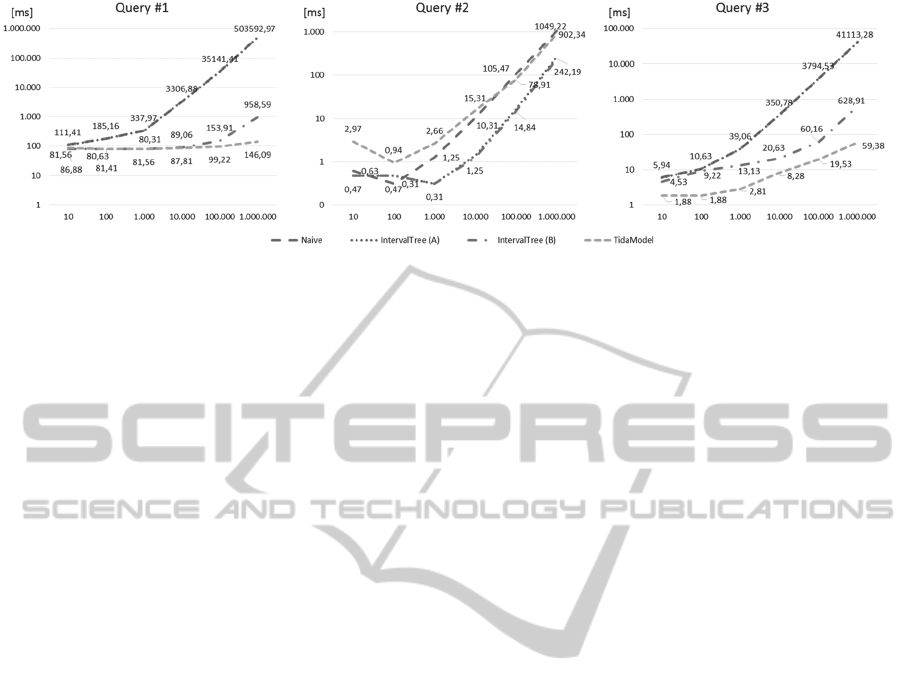
Figure 14: The measured average CPU-time performance (out of 100 runs per query).

vements:

1. The presented query language and its processing

do not support any type of transactions. A record

inserted, updated, or deleted is processed by the

system as an atomic operation. Nevertheless, roll-

backs needed after several operations have to be

performed manually. This generally increases im-

plementation effort on the client-side.

2. The presented XML definition of dimensions (cf.

3.3.1) uses regular expressions to associate a

member of a level to a descriptor value. Regular

expressions are sometimes difficult to be formal-

ized (especially for number ranges). An alterna-

tive, more user-friendly expression language is

desired.

3. The UPDATE and DELETE commands (cf. 3.4.1)

need the user to specify a record identifier. The

identifier can be retrieved from the result-set of an

INSERT-statement or using the SELECT REC‐

ORDS command. Nevertheless, users requested to

update or delete records by specifying criteria

based on the records’ descriptive values.

4. When a model is modified, it has to be loaded to

the system as new, the data of the old model has

to be inserted and the old model has to be deleted.

Users desire a language extension, allowing to up-

date models. Nevertheless, the implications of

such a model update could be enormous.

5 CONCLUSIONS

In this paper, we presented a query language useful to

analyze time interval data in an on-line analytical

manner. The language covers the requirements

formalized by several business analyst from different

domains, dealing with time interval data on a daily

basis. We also introduced four different implementa-

tions useful to process the most frequently used type

of query (i.e. SELECT TIMESERIES). An important

task for future studies is to confirm, or define new

models and present novel implementations solving

the problem of analyzing time interval data. In addi-

tion, future work should focus on distributed and in-

cremental query processing (e.g. when rolling-up a

level). The mentioned considerations (cf. section 4.3)

of our introduced language and its implementation

should be investigated. Another interesting area con-

sidering time-interval data is on-line analytical min-

ing (OLAM). Future work should study the possibili-

ties of analyzing aggregated time series to discover

knowledge about the underlying intervals. Finally, an

enhancement of the processing of the two-step aggre-

gation technique should be considered. Depending on

the selected aggregations an optimized processing

strategy might be reasonable.

ACKNOWLEDGEMENTS

The approaches presented in this paper are supported

by the German Research Foundation (DFG) within

the Cluster of Excellence “Integrative Production

Technologies for High-Wage Countries” and the pro-

ject “ELLI – Excellent Teaching and Learning in En-

gineering Sciences” as part of the Excellence Initia-

tive at the RWTH Aachen University.

REFERENCES

Agrawal, R. and Srikant, R., 1995. Mining sequential

Patterns, Int. Conf. Data Engineering, Taipei, Taiwan,

pp. 3-14.

Allen, J. F., 1983. Maintaining knowledge about Temporal

Intervals, Communication ACM 26, 11, pp. 832-843.

Böhlen, M. H., Busatto R., Jensen C. S., 1998. Point-versus

interval-based temporal data models, 14th Int. Conf. on

Data Engineering, Orlando, Florida, USA, 23.-27.

Feburary, pp. 192-200.

Chen, Y.-L., Chiang, M.-C., and Ko, M.-T., 2003. Disco-

TIDAQL-AQueryLanguageEnablingon-LineAnalyticalProcessingofTimeIntervalData

vering time-interval sequential patterns in sequence

databases, Expert Systems with Applications 25(3), pp.

343-354.

Codd, E. F., Codd, S. B., and C. T. Salley, 1993. Providing

OLAP (On-Line Analytical Processing) to User-

Analysts: An IT Mandate, E. F. Codd and Associates

(sponsored by Arbor Software Corp.).

Höppner, F., Klawonn, F., 2001. Finding informative rules

in interval sequences. Hoffmann, F., Adams, N., Fisher,

D., Guimarães, G., Hand, D.J. (eds.) IDA2001. LNCS,

vol. 2189, Springer, Heidelberg, pp. 123-132.

Kimball, R. and Ross, M., 2013. The data warehouse

toolkit: The definitive guide to dimensional modeling,

3rd Edition, Wiley Computer Publishing.

Kline, N. and Snodgrass, R. T., 1995. Computing temporal

aggregates, 11th Int. Conf. on Data Engineering (ICDE

1995), Taipei, China, 06.-10. March, pp. 222-231.

Koncilia, C., Morzy, T., Wrembel, R., and Eder J., 2014.

Interval OLAP: Analyzing Interval Data, Data

Warehousing and Knowledge Discovery (DaWaK

2014), Volume 8646, Springer Int., pp. 233-244

Kotsifakos, A., Papapetrou, and P., Athitsos, V., 2013.

IBSM: Interval-based Sequence Matching, 13th SIAM

Int. Conf. on Data Mining (SDM13), Austin, Texas,

USA, 02.-04. May.

Kriegel, H.-P., Pötke, M., and Seidl, T. (2001). Object-

Relational Indexing for General Interval Relationships,

7th Int. Symposium on Spatial and Temporal Databases

(SSTD 2001), Los Angeles, California, 12.-15. July, pp.

522-542.

Mazón, J.-N., Lichtenbörger, J., and Trujillo J., 2008.

Solving summarizability problems in fact-dimension

relationships for multidimensional models, 11th Int.

Workshop on Data Warehousing and OLAP (DOLAP

'08). Napa Valley, California, USA, 26.-30. October.

pp. 57-64.

Meisen, P., Meisen, T., Recchioni, M., Schilberg, D.,

Jeschke, S., 2014. Modeling and Processing of Time

Interval Data for Data-Driven Decision Support, IEEE

Int. Conf. on Systems, Man, and Cybernetics, San

Diego, California, USA, 04.-08. October.

Meisen, P., Keng, D., Meisen, T., Recchioni, M., Jeschke,

S., 2015. Bitmap-Based On-Line Analytical Processing

of Time Interval Data, 12th Int. Conf. on Information

Technology. Las Vegas, Nevada, USA, 13.-15. April.

Mörchen, F., 2006. A better tool than Allen’s relations for

expressing temporal knowledge in interval data, 12th

ACM SIGKDD Int. Conf. on Knowledge Discovery and

Data Mining, Philadelphia, Pennsylvania, USA.

Mörchen, F., 2009. Temporal pattern mining in symbolic

time point and time interval data, IEEE Symp. on Com-

putational Intelligence and Data Mining (CIDM 2009),

Nashville, Tennessee, USA, 30. March-2. April.

Pedersen, T. B. 2000, Aspects of data modeling and query

processing for complex multidimensional data, Ph.D.

thesis, Aalborg Universitetsforlag, Aalborg.

Publication: Department of Computer Science,

Aalborg Univ., no. 4.

Papapetrou, P., Kollios, G., Sclaroff S., and Gunopulos, D.,

2005. Discovering Frequent Arrangements of Temporal

Intervals, 5th IEEE Int. Conf. on Data Mining

(ICDM’05), IEEE Press, pp. 354-361.

Papapetrou, P., Kollios, G., Sclaroff S., and Gunopulos D.,

2009. Mining Frequent Arrangements of Temporal

Intervals, Knowledge and Information Systems, vol. 21,

no. 2, pp. 133-171.

Rafiei, D. and Mendelzon, A. O., 2000. Querying Time

Series Data Based on Similarity, IEEE Transactions on

Knowledge and Data Engineering, 12(5).

Spofford, G., Harinath, S., Webb, C., Huang, D. H., and

Civardi, F., 2006. MDX-Solutions: With Microsoft

SQL Server Analysis Services 2005 and Hyperion

Essbase, John Wiley & Sons, ISBN 0471748080.

ICEIS2015-17thInternationalConferenceonEnterpriseInformationSystems