An Economic Approach for Generation of Train Driving Plans using

Continuous Case-based Planning

Andr´e P. Borges

, Osmar B. Dordal

, Richardson Ribeiro

, Br´aulio C.

Avila

and Edson E. Scalabrin

Programa de P´os-Graduac¸ ˜ao em Inform´atica, Pontif´ıcia Universidade Cat´olica do Paran´a,

Rua Imaculada Conceic¸˜ao 1155, Curitiba, Paran´a, Brazil

Department of Informatics (DAINF), Federal University of Technology-Parana,

Via do Conhecimento, Km 1, Pato Branco, Paran´a, Brazil

Keywords:

Case-based Planning, Driving Plans.

Abstract:

We present an approach for reusing and sharing train driving plans P using continuous (or without human

intervention) Case-Based Planning (CBP). P is formed by a set of actions, which when applied, can move a

train in a stretch of railroad. This is a complex task due to the variations in the (i) composition of the train,

(ii) environmental conditions, and (iii) stretches travelled. To overcome these difﬁculties we provide to the

driver a support system to help the driver in this complex task. CBP was chosen because it allows directly

reuse the human drivers experience as well as from other sources. The main steps of the CBP are distributed

among specialized agents with different roles: Planner and Executor. Our approach was evaluated by different

metrics: (i) accuracy of the case recovery task, (ii) efﬁciency of task adaptation and application of such cases

in realistic scenarios and (iii) fuel consumption. We show that the inclusion of new experiences reduces the

efforts of both the Planner and the Executor, reduces signiﬁcantly the fuel consumption and allow the reuse

of the obtained experiences in similar scenarios with low effort.

1 INTRODUCTION

For years, different sectors of the economy have been

tested in relation to their innovation capabilities and

competitiveness, which can be summarized by the ex-

pression doing what we already do well, better. These

capabilities, in general, aim to create new cash ﬂows

for a company. Thus, the use of information tech-

nology is imperative for establishing a different and

sophisticated way to reduce costs without compro-

mising quality, and still consider the scarcity of re-

sources. In this scenario, the railroad, to be compet-

itive, must minimize transportation costs and capital-

ize every available resource, such as railroad cars and

locomotives.

Although the railroad is one of the most feasible

modes for freight transportation, there is still latitude

for cost reduction. The use of any technological re-

source that can reduce expenses, for example, fuel

consumption, can represent signiﬁcant cost reduction

in one year of operation. For example, the United

States of America railroads consumed 3.600 million

of gallons of fuel in 2012, approximated 145.7 thou-

sand gallons per locomotive, which represent a cost

14.285 mi of dollars (of the Assistant Secretary for

Research and of Transportation (US DOT), 2014).

The establishment of general train driving policies

that derive from important ﬁnancial returns is difﬁ-

cult because of: (i) the need (or existence) of special-

ized training for drivers; (ii) variations in train for-

mation (e.g., number of locomotives, railroad cars);

and (iii) inﬂuence of driving conditions (i.e., climate,

constraints). Moreover, the train driver must possess

signiﬁcant knowledge regarding rules and regulations

(e.g., driver cab controls, signaling systems, and track

safety), traction knowledge (e.g., engine layout and

safety systems) and route knowledge, in addition to

several hours of practical driver skills. This set of re-

quirements is necessary in order to achieve a feasible

safe, fast and cost-effective driving of several trains.

In this context, an approach for generating cen-

tralized driving plans that drive with static rules has a

small possibility of producing signiﬁcant results given

variations in the use conditions of the track and di-

versiﬁcation of the experiences gained. The approach

proposed here includes the use of a distributed archi-

tecture to increase the availability of resources such

as experiences and comprehensiveness of plans be-

440

P. Borges A., B. Dordal O., Ribeiro R., C. Ávila B. and E. Scalabrin E..

An Economic Approach for Generation of Train Driving Plans using Continuous Case-based Planning.

DOI: 10.5220/0005348504400451

In Proceedings of the 17th International Conference on Enterprise Information Systems (ICEIS-2015), pages 440-451

ISBN: 978-989-758-096-3

 2015 SCITEPRESS (Science and Technology Publications, Lda.)

fore and during execution of such plans. Further-

more, the application of case-based learning allows

those involved to become increasinglyspecialized and

autonomous. To achieve autonomy and specializa-

tion, the existence of some agents specialized in well-

deﬁned tasks is assumed: Memory (maintaining a

case base), Planner (preparingfeasible drivingplans),

and Executor (executing and adjusting plans).

The Planner and Executor agents adapt and exe-

cute plans, respectively, against different driving con-

ditions and strategies. For example, a given strategy

can target speciﬁc goals, such as energy efﬁciency or

driving speed. The construction base of each strat-

egy can be purely mathematical, algorithmic, or rule-

based (e.g., hIF-THENi) (Sato et al., 2012). These

techniques offer few possibilities for adaptation with-

out the intervention of an expert in this ﬁeld. Such dif-

ﬁculty represents an important limitation when there

is diversiﬁcation of the proﬁles of the railroads and

trains involved.

In this paper,the main motivation is to improve the

performance of Executor agents when facing new sit-

uations, by exchanging experiences between agents,

reducing the necessary efforts to apply a driving plan.

The exchange of experiences occurs when the ex-

ecuted driving plans by human drivers, or another

sources, is incorporated to the knowledge base of

Memory agent and is used by Planner agent to elabo-

rate new driving plans.

The driving plans are elaborated using the Case-

Based Planning approach without human interac-

tion. CBP is based on canonical case-based reasoning

(Aamodt and Plaza, 1994)(Spalzzi, 2001). This ap-

proach is divided in four main steps: recover the past

case solutions that are similar to the new problem,

reuse and adapt (if necessary) the most similar case,

revise the proposed solution to guarantee its applica-

bility and retain the new solution for future use. At

ﬁrst step, an Euclidian Distance is used by the Mem-

ory agent to calculate the distance between the new

problem and the stored cases. A set of most similar

cases will be adapted using the Genetic Algorithm,

which tries to optimize the new solution. The best

adapted solution is revised according to domain spe-

ciﬁc knowledge, to guarantee the safety during the

journey, avoiding situations that damage the train or

the railroad, like slipping, lack of moving force or

high speed. At end, the executed driving plans are

stored by Memory agent when it returns to the sta-

tion.

The approachwas evaluated by the accuracy of the

case recovery task, and the efﬁciency of task adapta-

tion and application of such cases in several scenarios.

The applicability of the proposed solution is evaluated

in terms of fuel consumption, comparing our best sce-

nario against the fuel consumptions obtained for other

approaches with the same conﬁgurations of train and

railroad. We show that the inclusion of new expe-

riences reduced the efforts of both the Planner and

the Executor and reduces signiﬁcantly the fuel con-

sumption. In addition, the CBR approach allowed the

reuse, with low effort, of the obtained experiences in

similar scenarios.

The next section introduces some related works.

Section 3 presents the developed system. Then, Sec-

tion 4 shows some of the experiment results. Finally,

the last section presents our conclusions.

2 RELATED PAPERS

Many researches have applied Case-based reasoning

within various problem-solving domains. For exam-

ple, like a recommender mechanism (Wang and Yang,

2012) or in autonomic systems to minimize human in-

tervention and to enable a seamless self-adaptive be-

havior in the software systems. (Khan et al., 2011).

Case-based reasoning has been used successfully

in collaborative systems whose missions were to as-

sist people in various tasks, such as selecting the

appropriate behavior for an unattended vehicle ride

(Bajo et al., 2007) (Vacek et al., 2007) , optimizing

industrial processes (Navarro et al., 2012), and estab-

lishing rules used to assist experts in detecting envi-

ronmental changes (Mota et al., 2008). In these sys-

tems, the goal was to share plans as a way of enrich-

ing experiences by generating shared and interactive

plans and execution. In our application, the collabora-

tive driving approach directly considered the experi-

ences of human drivers (adjusting them if necessary),

as well as the experiences of automatic driving sys-

tems. Also, our main difference lies in the indepen-

dent execution of the plan, i.e., during its execution,

there is no interaction with the Planner (which gener-

ated the plan) located in the processing station. The

Executor is embedded in the onboard computer of the

main locomotive,without a dedicated communication

channel with the agents of its origin station. There is

no transmission of driving plans because of environ-

mental restrictions, such as the presence of tunnels,

distance of transmission towers, and increase in the

cost of the operation.

In railroad transportation, several works were de-

veloped over the years in order to optimize driving

and use of the rail network. In (Gu et al., 2012)

the focus was to determine the speeds practiced dur-

ing the trip, using non-linear programming to avoid

abrupt actions from the driver agent. A similar focus

AnEconomicApproachforGenerationofTrainDrivingPlansusingContinuousCase-basedPlanning

441

TATION

PA Planner Agent

EA Executor Agent

Dispatcher

<Ei-1, Ei>

Control

Comunication

Case

Base

Memory Agent

<Ei, Ei+1>

Figure 1: ITDS: Representation of a station, with a Memory

agent, two Planner agents, and two Executor agents.

was given by (Hengyu and Hongze, 2012), but with

the use of fuzzy neural networks to control actions.

In (Fang et al., 2013) the authors present several ap-

proaches developed for re-scheduling problem in rails

networks. In (D. and Houpt, 2011) the authors present

a train control-system to optimize trips that requires

the continuously proﬁle update by GPS (Global Posi-

tioning System) to control the locomotives, however,

due the presence of tunnels the GPS signal may fail

and become unavailable. Finally, in (Borges et al.,

2012) a single agent, based on CBR, was created to

prepare train-driving plans based on the recovery of a

single action at a time. The internal organization of

the case base was proposed in the composition of the

cases and specializations, which required time to be

organized, and resulted in lower percentages of suc-

cess than those presented here. Furthermore, the plan-

ning of a single action at a time made the approach

computationally costly.

3 ARCHITECTURE

The developed system, referred to as the Intelligent

Train Drive System (ITDS) utilizes the following re-

sources: rail network, freight train, and software

agent (Wooldridge and Jennings, 1995). The rail net-

work is viewed as a graph where the vertices repre-

sent physical or logical stations, and the edges have

information from the track (i.e., proﬁle). Each station

hosts a Memory agent, a Planner, and one or more

Executors for each stretch S

. This conﬁguration is il-

lustrated in Figure 1, where the triple hE

i−1

i+1

deﬁnes the ends of two stretches S

= hE

i−1

i and

= hE

i+1

The interaction between the different agents is

well deﬁned in time. Planner PA1 receives, from an

external system, a demand d to drive the train on a

stretch S

. PA1 then segments plan P of stretch S

into

n parts p

,..., p

, according to the vertical proﬁle of

the stretch. The cycle starts. For each p

, PA1 for-

wards to Memory agent MA1 a request for plans ap-

plicable in p

. MA1 collaboratively returns to PA1 a

set of candidate plans SP = sp

,...,sp

. PA1 reduces

this set SP to a single feasible plan sp

, adapting it

to the current situation, and includes sp

in plan P.

Then, it selects p

k+1

and repeats this cycle n times.

At the end, P is forwarded to an EA1, which embarks

on the train and applies it.

During the application of P, there is no com-

munication between the agents, a differential aspect

when compared to other approaches (D. and Houpt,

2011)(Gu et al., 2012)(Hengyu and Hongze, 2012).

However, because the conditions for plan execution

may change, it may be necessary to partially redo

parts of plan P. The capacity of the Executor to redo

parts of plan P ensures feasible and safe driving with-

out the need to receive a new plan from PA1. This

is an important aspect for making the use of commu-

nication channels less relevant. Existing train-station

communication is only used for monitoring and con-

trolling the position of each train. This helps to reduce

the costs of freight transport and coupling across sys-

tem software modules.

The algorithm 1 summarizes the ITDS ﬂow. The

input of the algorithm is a base-case B containing past

experiences of human drivers or another fonts. While

a demand is not emitted by a Dispatcher, the system

remain waiting for a demand (lines 1-3). When the

order is received, the Planner elaborates a plan P to

attend the d using the previous experiences stored in

B (line 4). Next, the Executor agent will execute P

(line 5). After the execution of P, the executed plan P

′

is incorporated in the case-base of the Memory Agent

(line 6).

Algorithm 1: Basic ITDS ﬂow.

Require: a case-base B

1: while d = null do

2: d ← listenDispatcher()

3: end while

4: P ← planner(B, d)

5: P

′

← execute(P)

6: B ← store(B,P

′

)

The agents responsible for execute the tasks sum-

marized will be described in the next section.

3.1 Agents

The role of the Dispatcher is to globally manage the

times and orders for the movement of trains in a rail

network, rationally attempting to occupy the spaces

ICEIS2015-17thInternationalConferenceonEnterpriseInformationSystems

442

and existing resources (Company, 1979). The Dis-

patcher decides whether to stipulate the maximum al-

lowable speed at certain points of the track, and to

restrict or allow the passage of the train in a sec-

tor (Company, 1979). This information is sent to

the Planner along with the dispatch order, trigger for

planning.

The Planner generates a driving plan P to meet the

demand of the Dispatcher, which is to move train T

from end E

to E

i+1

. Each action of P can take one of

the following behaviors: accelerate, maintain, or re-

duce the speed of train T. Each behaviour is adjusted

according to a speciﬁed power. Accelerate and reduce

correspond, respectively, to increase and decrease ac-

celeration points. In a locomotive, each acceleration

point, typically from 1 to 8, generatesa positive power

capable of moving the train. Speed reduction can be

accomplished by generating a power less than the sum

of the resistances or by applying the brakes. Brak-

ing involves applying pressure in the brake pipe, mea-

sured in psi (pressure in pounds per square inch) and

is represented here by acceleration point -1. To move

the train, an appropriate acceleration point for a given

position of the railroad stretch to be covered must be

planned in order to avoid sliding and overcome the

sum of resistances (Loumiet et al., 2005).

To ensure train movementin all points of the track,

it is also necessary to know the minimum required

power. This power is calculated by the Dispatcher and

reported to the Planner in the dispatch order. The cal-

culation considers the minimum tractive force of all

the locomotives intended to move a train against the

high resistance of the stretch to be covered. Moreover,

the resulting set of actions should meet the objectives,

which are in opposition in the ﬁrst two at the base, of

performing a quick trip, reducing fuel consumption,

and complying with the security restrictions. Thus,

one should plan speeds near the cruise speed, for ex-

ample, 5 km/h below the maximum speed. Within this

criterion, actions should reduce fuel consumption and

travel time. The resulting set is the driving plan P for

train T in a stretch S.

The role of the Executor is to apply plan P, re-

ceived at end E

, performingthe following basic tasks:

testing the applicability of ak based on the current

train conditions, adjusting the parameters of a

(if

necessary), and applying a

. Until the complete ex-

ecution of P, P may undergo several ∆ adjustments.

For example, in the case of non-applicability of an

action a

, the Executor may adjust ak based on driv-

ing skills. Adverse conditions may represent, for ex-

ample, a climate change (changes the friction coefﬁ-

cient), changes in the maximum allowable speed, and

others. Such conditions perceived by various sensors

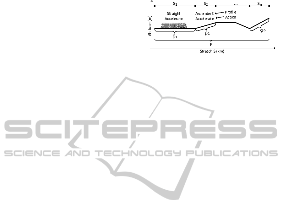
Figure 2: Example of segmentation of a stretch S into parts

,...,s

according to the vertical proﬁle and a set of cases

, p

,..., p

, which when ordered form a plan P for the

movement of trains.

are read in predetermined time intervals.

The Memory agent has two basic functions: (i)

providing the Planner with a set of plans applicable

to each part of a given stretch and (ii) maintaining a

base of plans in a dynamic memory structure (Schank,

1983). Each Memory, located in a station, maintains

only the plans applied in the stretches from ends E

to E

i+1

and from E

to E

i−1

. Maintaining only the

plans of the stretches connected to the station allows

specialization in these stretches. Each plan executed

P+ ∆ is returned to the Memory of the origin end

point to be integrated into the local base of the sta-

tion plans. Such structure allows the inclusion of a

new plan that can activate simple internal processes

of plan reclassiﬁcation and/or more sophisticated op-

timization of data structures and indexing of plan con-

tents (Schank, 1983).

3.2 The Plan Elaboration

The elaboration of a plan requires: information from

the train (i.e., position, number of locomotives and

railroad cars, and weight) and from the track stretch

(i.e., maximum speeds, friction coefﬁcients, and ver-

tical proﬁle). The vertical proﬁle is critical for deﬁn-

ing the relevant portions of a stretch S = s

,...,s

(see

Figure 2).

For each part s

, a plan is prepared that corre-

sponds to a new problem to be solved. Each part

must become specialized. Figure 2 illustrates plan

P with p

,..., p

. Each p

describes a set of actions

with more predictable behaviours (maintain, acceler-

ate, and reduce) for a vertical proﬁle (rising, falling,

and plain/plateau).

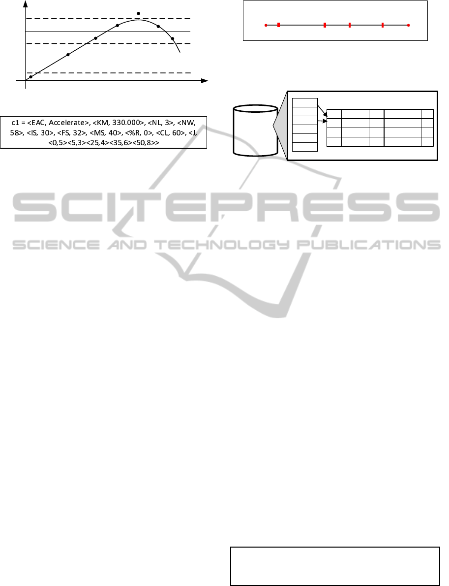
The behaviours that must be undertaken for proper

driving are shown in Figure 3. Such behaviours will

vary depending on current speed s, initial speed s

cruise speed s

, and maximum speed s

(Pinto et al.,

1985). Proper driving is obtained when the current

speed is greater than the initial speed and less than

the maximum speed, remaining close to the cruis-

AnEconomicApproachforGenerationofTrainDrivingPlansusingContinuousCase-basedPlanning

443

III

critical

Figure 3: Possible states of train driving (Pinto et al., 1985).

Figure 4: Example of a retrieved case.

ing speed. States indicate actions that must be per-

formed to achieve proper driving. State I suggests

ACCELERATING the train because the current speed

is less than the initial speed. States II and III

suggest

ACCELERATE or MAINTAIN speed. On the other

hand, state III

must REDUCE the speed because of

the proximity to the current speed with the maximum

speed. In state IV, it must ACCELERATE to approx-

imate the current speed to the speed regimen. The

BRAKING action is recommended in stateV because

the train can exceed the maximum allowable speed.

Pragmatically, case C is a representation of a real-

world object or episode in a particular representation

scheme (Kolodner, 1993). A case represents a ﬁnite

set of n attribute/value pairs that is a snapshot of the

situation executed by a train conductor during one

trip.

Figure 4 shows an example of a case recovered

in the form of pairs hattribute,valuei formed by the

following attributes: action performed (EAC), initial

kilometre (KM), number of locomotives (NL), num-

ber of railroad cars (NW), initial speed (IS) in km/h,

ﬁnal speed (FS) in km/h, maximum speed (MS) in

km/h, ramp percentage (%R), and total displacement

(CL) in meters. Although such attributes are pre-

sented as an illustration, they represent the dominant

features in the movement of a train.

A case also has a solution formed by a set

J = hm

,AP

i,hm

,AP

i,,hm

,AP

of ordered pairs. Each pair contains an acceleration

point (AP) and an application position (M) deﬁned in

meters. Figure 5 shows an instance of P, and an appli-

cation of each AP, from left to right, must move from

0 km to 60 km. The determination of each element of

P should allow the Executor to move the train safely

and efﬁciently.

It is expected that, as the Memory agent has in its

case base, a number of cases applied in stretches leav-

km x km x+60

5 3

Figure 5: Example of the solution of an applicable case in

kilometre (km) x to the maximum kilometre x+ 60.

Agent

Memory

Case Base

<PA1, EA1>

<PA1, EA2>

<PA2, EA1>

<PA2, EA2>

...

Case 1

Case 3

Case 8

Case 5

...

Plan <PA1, EA2>

Case 1

Profile

Straight

Action

Accelerate

...

Figure 6: Representation of the local Memory (left) case

base and example of part of a stored plan (right).

ing the station where it resides, there are greater pos-

sibilities of recovering an applicable case. If the case

is not fully applicable, it is believed that the adap-

tations are in reduced percentages. Figure 6 shows

the cases organized according to the actions taken (AP

and Action) and the constituents of the track proﬁle.

This organization allows recovery of cases more simi-

lar to the stretch of the track in question and the action

to be applied.

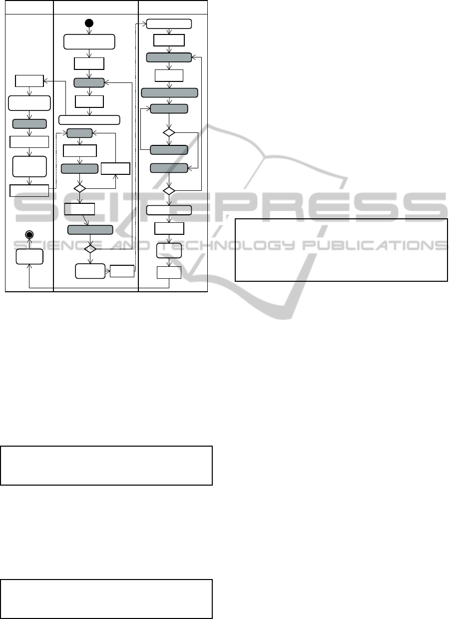
3.3 Inter and Intra Agents Data Flow

Figure 7 shows the basic ﬂow of inter and intra agent

collaboration. In this ﬁgure, the Dispatcher has been

omitted. Thus, the ﬂow is started by the Planner,

whose ﬁrst activity is to receive the dispatch order

generated by the Dispatcher and to generate a new

problem. As a result, two collaboration cycles are

established: the ﬁrst interactively involves the Plan-

ner agent and the Memory agent, and the second se-

quentially involves the Planner, Executor, and Mem-

ory. Henceforth, PA1 is used to designate a Planner

agent, EA1 an Executor agent, and MA1 a Memory

agent.

3.3.1 Planning Flow - Planner and Memory

Interaction

Planning starts when PA1 receives a dispatch order

from the Dispatcher.

(inform :sender Dispatcher :receiver PA1

:content (locomotives=3, wagons=58, [...]))

Then, the perception of the environment is per-

formed, resulting in a new case c1 to traverse stretch

ICEIS2015-17thInternationalConferenceonEnterpriseInformationSystems

444

Executor Agent (EA)Planner Agent (PA)Memory Agent (MA)

Revise

Recieve a dispatch

order

Retrieve

Request similar case

[retrieved]

C : Set<Case>

Reuse

[suggested]

c2 : Case

[valid?]

Retain in plan

[yes]

[no]

Recieve the plan

Retrieve action

Revise action

[yes]

Reuse action

[no]

Apply action

[end of trip?]

[no]

Finalize trip

[yes]

Send

Plan

[end of plan?]

Percept

[no]

Send plan

[yes]

[valid?]

[executed]

P : Plan

Read recieved

case

[new]

c1 : Case

Send set of

cases

[executing]

P : Plan

[planned]

ai : Action

Percept Environment

[new]

: Problem

Update

Base

<<asynchronous>>

[full]

P : Plan

[sent]

P : Plan

[new]

c1 : Case

[sent]

C : Set<Case>

[reproved]

c2 : Case

[approved]

c2 : Case

Figure 7: Basic ITDS ﬂow.

. The instantiation of c1 is managed by a dedicated

module that performs two basic functions: (i) read

sensors for speed, position, traction, and others, of the

train; (ii) calculate, in this case, the values for resis-

tance, effective tractive force of the pulling locomo-

tives, acceleration force, adherent tractive force, etc.

The data set (perceived and derivatives) deﬁnes the

values used to move the train (Loumiet et al., 2005).

PA1 passes on the new case instantiated by means

of a request to MA1.

(request :sender PA1 :receiver MA1 :content

(hattributes of the problemi))

Internally, the message is received and managed

by the Memory. The recovery of similar cases is done

using the Euclidian distance. The advantage of this

division of labor is to allow PA1 to perform another

task during the recovery phase, for example, to pro-

cess another dispatch order.The recovered cases are

then sent to PA1.

(inform :sender MA1 :receiver PA1 :content

(hset of similar casesi))

The most similar case c

is selected and adapted

according to the current perception (if necessary) by

the Reuse activity. This task involves replacing the

values of the J pairs (e.g., Figure 5), which are, re-

spectively, happlication position, acceleration pointi.

The adaptation step of the Planner used a genetic al-

gorithm (Baeck et al., 2000) (Mitra and Basak, 2005).

In a genetic algorithm the case base form the ini-

tial population of genotypes. Firstly, the algorithm

retrieves partial matching cases from case base with

speciﬁed design requirements. In this paper, each in-

dividual is composed by the recovered case solution J

and the initial population consist of the 50 most simi-

lar cases recovered from the Memory.

Next the retrieved cases are mapped into a geno-

type representation, so, the solution J of the each re-

covered case is mapped into a genotype of an individ-

ual, using integer numbers. For example, the individ-

ual of Figure 5 is mapped as

Individual Number: i0|

Evaluated: T

Fitness: f1138065562|427.0047|

i0|i5|i5|i3|i25|i4|i35|i6|i50|i8|i60|i8

to obey the standard used by the ECJ framework.

Later crossover and mutation operators are ap-

plied. The mutation and crossover rates are 50% for

both. We used one-point crossover since this tech-

nique have been good results when compared with

others (Magalh˜aes Mendes, 2013). Finally, newly

generated genotypes are mapped into corresponding

phenotypes/cases by inferring values for the attributes

and adding the context of the new design.

Applying the genetic algorithm to case adaptation

also requires the identiﬁcation of a ﬁtness function.

In this paper, two of the main objectives are to reduce

the fuel consumption and optimizing the speed prac-

tised by Executor agents. So, the ﬁtness function g(x),

illustrated in Equation 1, was deﬁned to minimize

such objectives, although they are opposites. These

attributes have a great impact on the generation of in-

dividuals and will determine their utility in the pop-

ulation. Each attribute has a factor which represents

his weight in the problem: fuel consumption ( flgtt)

and speed (fv), where flgtt = 0.02 e f v = 0.01. The

valuesof fuel consumption (lgtt) and speed (v) are ob-

tained by simulating the application of the individual

in the problem. During the simulation, the following

values are calculated for each action: consumption,

travel time, resistance, force to drive the train, and

others. Therefore, the ﬁtness function considers cal-

culations that result in the forces required to move the

train considered (Borges et al., 2012).

AnEconomicApproachforGenerationofTrainDrivingPlansusingContinuousCase-basedPlanning

445

Min.g(x) =

∑

j=0

(( flgtt × lgtt

) + ( fv× v

)) (1)

The values of f lgtt and fv were calculated by a

genetic algorithm made speciﬁc for it, where the indi-

viduals are composed by pairs of < flgtt, f v >. Each

parameter can vary according the interval [0.01;1.00],

totalling 100 possible values for each factor, being

this the value of each population generated by the

algorithm. For each individual a journey was simu-

lated, all with the same train and railroad conﬁgura-

tions. The fuel consumption obtained in each journey

was used as ﬁtness function value. The crossover and

mutation techniques used the same conﬁguration de-

veloped for this paper. The stopping criteria was set

to 100 generations, because there is a 10000 possible

factor combinations.

Returning to the adaptation step of this paper, the

crossover and mutation operations creates individu-

als that consists of solutions for the actual problem,

called proposed solutions. Each solution generated

by the genetic algorithm J is composed by accelera-

tion points and places of its applications, according to

Figure 5. Each proposed solution J is simulated, ap-

plying the acceleration points at the positions speci-

ﬁed in J. The resulting fuel consumption corresponds

to the ﬁtness of the individual. If the proposed solu-

tion is not applicable, because it results in slipping or

lack of movement force, the individual is penalized

with a high value for the ﬁtness and this individual is

discarded. The stopping criterion of the strategy was

the number of generations, equal to 10. At end, the

individual with minor value of ﬁtness will be chosen

for the adapted case. The ﬁtness function maximizes

some value by default, so, to minimize the fuel con-

sumption we convert the ﬁtness function to 1/g(x).

The adapted case c

′

i (corresponds to case c2 in

Figure 8) is feasible if and only if all parts of J meet

the following situations: (i) does not result in sliding,

(ii) have sufﬁcient force to move the train, and (iii) if

the acceleration point can be reduced and continue to

move the train, which indicates unnecessary fuel con-

sumption of the action. If the case is not approved,the

values of J are again submitted to the Reuse step, and

this is repeated until a valid solution is found and the

case is approved. A valid solution must comply with

the criteria (i) and (ii) described in the previous para-

graph, but not necessarily with criterion (iii), added

only to reduce fuel consumption.

After adding the valid adapted case in P, PA1 ver-

iﬁes whether the application of the plan results in the

arrival at the destination. If not, the planning cycle is

repeated for the next part of stretch s

. If so, P is sent

to EA1.

Figure 8: Adapted Case.

(execute :sender PA1 :receiver EA1 :content (the

plan P))

EA1 is embedded in the onboard computer of the

main locomotive and begins to command it. If later,

another train passes through the same station, another

Executor EA2 is created with a speciﬁc plan for the

new train.

3.3.2 Flow of Execution of the Plan - Executor

The plan execution cycle is similar to the planning

cycle. Each Executor starts its activities upon receiv-

ing the trip plan P. In possession of P, EA1 starts

the trip. During the trip, EA1 Recovers an action

of P and evaluates its preconditions. For such, it

perceives the environment through data read from the

onboard computer of the lead locomotive (e.g., max-

imum speed, friction coefﬁcient, and others). If no

precondition is violated at the time of reading, the a

action is applied, resulting in new information (i.e.,

speed, position, and others), which becomes the pre-

condition for the next action a

k+1

. On the other hand,

if one or more preconditions are invalid, for example,

because of some unforeseen event (e.g., rain, fog, or

changing the speed limit), EA1 corrects the action of

the plan based on its knowledge of driving (Reuse).

Such adjustment is made by evaluating the reason for

the failure, which can be: sliding, lack of force to

move, or stopping unexpectedly. It is expected for

each change (when required) to cause as insigniﬁcant

an impact as possible, i.e., the shortest distance be-

tween the planned and the applied acceleration point,

thus resulting in a reduced state space search.

Once the task of EA1 driving the train from end

to end E

i+1

is complete, the Finalize trip activity

is executed. In it, plan P and its ∆ adjustments are

processed, resulting in a plan P. P is returned to the

origin station E

by an Executor whose destination is

(inform :sender EA1 : receiver MA1 :content(an

executed plan P + ∆

The transport of the modiﬁed plan to the origin by

means of another train is assumed because, during the

trip, no communication channel is used to transmit the

ICEIS2015-17thInternationalConferenceonEnterpriseInformationSystems

446

plans between the train and the station. If the stretch

has only one direction, the plan is stored at the station

and forwarded to the next station that has a connec-

tion with the plan origin station. Communication be-

tween train and origin station is limited to sending in-

formation related to the conditions of the railroad and

the position of the train because of the cost of data

transmission and limitations of the means of commu-

nication, most of the time, against geographical con-

ditions.

3.3.3 Update Case Base - Memory

Memory agent MA1, upon receiving plan P, does the

following: for each proﬁle p

of P, identify the action

taken (accelerate, maintain, or reduce) based on the

speed variation practiced. Each separate and identi-

ﬁed part of the plan is compared with other existing

cases in the base. If it is already present, its reputation

receives a backup. Otherwise, a new event is inserted.

The reputation is a piece of information that allows

management of the case base (if necessary, thus re-

ducing the number of cases).

4 EXPERIMENTS

The approach was evaluated by different metrics: (i)

fuel consumption (LGTT), (ii) accuracy of the case

recovery task, and (iii) efﬁciency of task adaptation

and application of such cases in synthetic scenarios

which were created inspired in real-world scenarions.

The last two indicate the efﬁciency of the collabora-

tion of the Memory and Planner agents.

The experiments were conducted in a simulated

driving environment, and ﬁeld equations (Loumiet

et al., 2005) were implemented in Java (Luke et al.,

2014) and validated using several experiments. The

proﬁles of the railroads, trains, and the initial case

base are derived from real situations.

Table 1 deﬁnes the conﬁgurations of the trains

used in the experiments. To complete the experi-

ments, two different stretches of real railroads were

included: S

and S

, both with the same length (ap-

proximately 64 km), but with different proﬁlesvertical

and horizontaland maximum speed restrictions.

To evaluate the learning curve of each agent and

the performance of the collaboration in terms of shar-

ing and reusing plans, four scenarios were deﬁned

(see Table 2).

The initial case base of the Memory agent, in all

tested scenarios, contains actual trip plans and trips

executed in simulators (Sato et al., 2012).

Table 1: Train conﬁguration used in the experiments.

Train Locomotives Railway cars Weight (tons)

1 3 58 6278

2 4 100 6342

3 4 58 6541

4 2 31 3426

5 3 47 5199

6 2 31 3441

7 4 59 6579

8 2 28 3118

Table 2: Simulated scenarios in the experiments.

Scenario Train (Table 1) Reuse plans Stretch

A 1 No S

B 1 Yes S

C 1 Yes S

D [1;8] Yes S

The scenarios are evaluated according to the ef-

ﬁciency (%) of the recovery and adaptation steps of

the cases. This percentage indicates the success of re-

covery or adaptation of a case. For example, at any

given time, the Memory agent recovers, for the Plan-

ner agent, a case with a set of actions A = {3,4,4, 4}.

This set is adapted by the Planner, resulting in A =

{4,4,4,4}. Thus, the recovery task has an accuracy

of 75%. Then, A is passed to the Executor agent and

applied without any changes, resulting in a 100% ﬁt-

ting accuracy. Soon, the adaptation effort is 25% and

the execution effort, in terms of adaptation, is null.

In scenario A, the Memory agent uses only the ini-

tial case base. Ten trips were planned and all of them

for train 1 in stretch S

. All plans were executed by

an Executor agent. At the end of each trip, the new

experiences (new plans) were not incorporated to the

case base of the Memory agent. Figure 9 presents the

efﬁciency (%) of the recovery and adaptation steps of

all the cases in the ten trips. It is observed that the

recovery of cases is less effective than the adaptation

of cases. In percentage, the difference between the

recovery and adaptation task corresponds to the con-

tribution of the adaptation task to make the plan appli-

cable to a given case. The average of this difference

is 8%, with a standard deviation of 1%. Compared

to a method of satisfaction of constraints, the effort

obtained is less in terms of memory used, execution

time, and number of states. Regardless of the highest

peaks of success of the recovery and adaptation task

being 46% and 51%, respectively, the generated and

executed plans are similar at 86%. The similarity is

calculated by the Cosine distance.

In scenario B, the same train conﬁguration and

the same stretch from scenario A was used. How-

ever, at every trip made by the Executor agent, the

applied plan was incorporated to the case base of the

AnEconomicApproachforGenerationofTrainDrivingPlansusingContinuousCase-basedPlanning

447

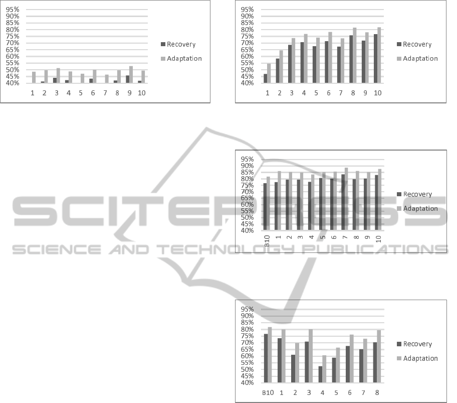
Figure 9: Results of scenario A. Ten trips with the same

train conﬁguration (conﬁguration 1), in stretch S

and with-

out reusing plans.

Memory agent. Figure 10 shows that the inclusion

of new plans in the case base of the Memory agent

increased by approximately 25% the efﬁciency of the

recovery and adaptation tasks. The similarity between

what was planned and what was executed is on aver-

age 90%. The addition of new cases to the experience

base broadens the efﬁciency of the planning task. It

is observed that between trips 1 and 3, there is an

increasing linear trend of 20%. Moreover, from trip

3, there is a slightly increasing stability, with average

variation of 4% for both tasks, and with standard de-

viation of 2%. The variation is justiﬁed because the

trips followed speeds similar to each other, but with

differences in driving plans at certain times. This dif-

ference occurs because of adaptations made by the

genetic algorithm, which in some places suggested

different acceleration points. This results in variation

in the power used, and consequently, variation of the

practiced speeds. This fact is inherent to the natural

behavior of the genetic approach (e.g., mutation).

In scenario C, as in scenario B, on each new trip

made by the Executor agent, the applied plans are in-

corporated into the experience base of the Memory

agent, and thus reused by the Planner agent. The

case base of the Memory agent began with the experi-

ences generated in scenario B. The steps for recovery

and adaptation have an average efﬁciency of 80% and

86%, respectively (see Figure 11).

In percentage, the difference between the recov-

ery and adaptation task was 9% at the beginning of

the experiment, and then immediately fell to an av-

erage of 5%, with a standard deviation of 1%. De-

spite increased effort because of unfamiliarity with

the environment, the results are signiﬁcant. These re-

sults encourage the use of a collaborative approach

between agents, located at different stations, to ex-

change plans.

Figure 12 shows the results of scenario D, where

the trips always occur in the same track, but with eight

different train formations. In this scenario, the Mem-

ory agent initiates the experiences of scenario B. In

Figure 10: Results of scenario B. Ten trips with the same

train conﬁguration (conﬁguration 1), in stretch S

and

reusing implemented plans.

Figure 11: Results of scenario C. Same train conﬁgura-

tion (conﬁguration 1) and initial plans of scenario B, but

in stretch S

Figure 12: Results of scenario D. Different train conﬁgu-

rations (conﬁgurations 1 to 8), initial plans of scenario B,

stretch S

terms of efﬁciency of recovery and adaptation tasks,

the adaptation task proves superior. There is an ex-

pected drop in success because the train conﬁgura-

tions are different for each trip. However, even in this

scenario without repetition of train conﬁguration, it is

possible to note that, to the extent that new cases are

included in the base, the overall efﬁciency improves.

Hopefully, with a greater number of trips with similar

conﬁgurations, efﬁciency rates move rapidly towards

scenario B.

In the scenarios on which we worked, it can be ob-

served that without reusing plans as past solutions, the

average success rates in the recovery and adaptation

tasks remain low, 42% and 49%, respectively. How-

ever, when we start to reuse the plans as past solu-

ICEIS2015-17thInternationalConferenceonEnterpriseInformationSystems

448

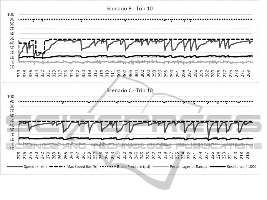
Figure 13: Data of trips made for the same train conﬁguration in different stretches.

tions, the average success rates of recovery and adap-

tation tasks increase to 64% and 74%, respectively.

In terms of complexity, raising the efﬁciency of such

tasks reduces the effort of searching for the problem

solution. Finally, the contribution of the adaptation

task, in the reuse of shared experiences of different

stretches, remained at the same level of scenario B.

This suggests that the accumulation of cases in a given

scenario proves to be useful in another scenario.

Figure 13 shows graphically the execution of the

ten trips for scenarios B and C. It can be noted that

there is a signiﬁcant difference for each proﬁle. Such

differences can be observed in the maximum speeds

practiced, percentages of ramps, and resistances. The

evolution of the speeds shows a signiﬁcant difference

in driving style. The decrease in speeds is related to

the applications of the brakes, and to reﬂections of

the driving policy that attempts to maintain the speed

of the train near the maximum allowable speed. Such

heuristics are applied to attempt to reduce the duration

of a trip. It should be indicated that the ﬁrst appli-

cation of the brake follows a default value and must

heavily inﬂuence train speed. A smoother speed re-

duction without exceeding the safe speed limit is de-

sired. Such a study is not part of this paper, but it can

be incorporated into the Planner agent, thus giving it

a look ahead mechanism.

In general, in all observed situations, the effort on

adaptation is present, but efﬁcient, and rises over time.

For the ﬁeld in question, as the trains and the environ-

ment change, the plans used in past situations are not

easily applicable to others; this effectively requires an

adaptive and efﬁcient approach. This ﬁnding goes to

the direction of what has classically been understood

as an advantage of the CBR approach in view of a

rule-based approach (Kolodner, 1993). The latter ap-

proach requires explicit knowledge models regarding

the application domain. This demand is difﬁcult to

execute in a complex environment. It also fails when

there is no rule that can be applied in the ﬁeld. Fur-

thermore, if the environment changes, there is a need

to update the rule base to be able to derive a solution.

As in CBR, knowledge of the ﬁeld is represented in

the form of cases. It exempts an explicit representa-

tion of the application domain. This allows dynami-

cally maintaining and learning new knowledge as new

cases are incorporated into the case base.

Table 3 is a comparison table that contrasts the

performance of human drivers (Actual column) driv-

ing a simulator where the actions applied are deter-

mined by a constraint satisfaction system (DCOP col-

umn) (Sato et al., 2012) and by the approach pre-

AnEconomicApproachforGenerationofTrainDrivingPlansusingContinuousCase-basedPlanning

449

Table 3: Consumptions obtained in scenario C.

Train

Consumption (LGTT) Reduction

Actual DCOP Our C-A C-B

(A) (B) (C) (%) (%)

1 6.19 4.16 3.36 50% 26%

2 5.68 4.18 4.22 30% -5%

3 6.23 4.09 3.95 41% 10%

4 6.49 4.51 3.88 46% 23%

5 6.29 4.22 3.31 49% 24%

6 6.17 3.99 3.69 40% 8%

7 6.26 4.07 3.86 42% 11%

8 5.68 4.41 4.00 34% 6%

sented (Our column). The DCOP column represents

the best values obtained in this approach. It is em-

phasized that for all consumption values (measured

in LGTT), our approach is higher than for the other

competitors, except on a single opportunity (train 2),

where the DCOP is higher by 5%.

The feasibility of an automatic train driving sys-

tem seems signiﬁcantly important. For example, for

a fuel consumption expenditure of approximately 250

million dollars per year, any cost savings above 6%

can have a signiﬁcant impact on the competitiveness

of the freight transport sector.

5 CONCLUSIONS

This paper presented a collaborative approach for

sharing experiences in generating plans for driving

trains. The results obtained showed that the adopted

approach can be generalized and deployed at various

stations of a rail network. We showed that the efﬁ-

ciency of recovery and adaptation tasks increases as

new cases are obtained. Such efﬁciency generates a

tendency to reduce efforts in planning and re-planning

driving plans. Obviously, if conditions change signif-

icantly, planning efforts increase, at least initially.

Finally, in terms of domain application, two re-

sults are important: in monetary terms, the gener-

ated driving plans can produce signiﬁcant gains; and

in terms of reuse of experiences, the approach sug-

gested that good drivers should be used to drive trains

in several different stretches of a railroad, for a certain

time, in order to generate experiences. Such experi-

ments can then be used to generate good plans for less

experienced drivers. This helps rationalize the exper-

tise capable for driving trains efﬁciently. Future work

should follow the following directions: avoiding un-

necessary stops (Dordal et al., 2011), and ensuring the

certiﬁcation of the information exchanged.

REFERENCES

Aamodt, A. and Plaza, E. (1994). Case-based reasoning:

Foundational issues, methodological variations, and

system approaches. AI Commun., 7(1):39–59.

Baeck, T., Fogel, D., and Michalewicz, Z. (2000). Evolu-

tionary Computation 1: Basic Algorithms and Opera-

tors. Basic algorithms and operators. Taylor & Fran-

cis.

Bajo, J., Corchado, J., and Rodr´ıguez, S. (2007). Intelli-

gent guidance and suggestions using case-based plan-

ning. In Weber, R. and Richter, M., editors, Case-

Based Reasoning Research and Development, volume

4626 of Lecture Notes in Computer Science, pages

389–403. Springer Berlin Heidelberg.

Borges, A., Dordal, O., Sato, D., Avila, B., Enembreck,

F., and Scalabrin, E. (2012). An intelligent system

for driving trains using case-based reasoning. In Sys-

tems, Man, and Cybernetics (SMC), 2012 IEEE Inter-

national Conference on, pages 1694–1699.

Company, G. R. S. (1979). Elements of railway signaling.

General Railway Signal.

D., E. and Houpt, P. (2011). Trip optimizer for railroads.

Technical report, IEEE Control Systems Society.

Dordal, O., Borges, A., Ribeiro, R., Enembreck, F., Scal-

abrin, E., and Avila, B. (2011). Strong reduction in

fuel consumption driving trains in bi-directional sin-

gle line using crossing loops. In Systems, Man, and

Cybernetics (SMC), 2011 IEEE International Confer-

ence on, pages 1597–1602.

Fang, W., Sun, J., Wu, X., and Yao, X. (2013). Re-

scheduling in railway networks. In Computational In-

telligence (UKCI), 2013 13th UK Workshop on, pages

342–352.

Gu, Q., Cao, F., and Tang, T. (2012). Energy efﬁcient

driving strategy for trains in mrt systems. In Intelli-

gent Transportation Systems (ITSC), 2012 15th Inter-

national IEEE Conference on, pages 427–432.

Hengyu, L. and Hongze, X. (2012). An integrated intel-

ligent control algorithm for high-speed train ato sys-

tems based on running conditions. In Digital Man-

ufacturing and Automation (ICDMA), 2012 Third In-

ternational Conference on, pages 202–205.

Khan, M. J., Awais, M. M., Shamail, S., and Awan,

I. (2011). An empirical study of modeling self-

management capabilities in autonomic systems using

case-based reasoning. Simulation Modelling Practice

and Theory, 19(10):2256 – 2275.

Kolodner, J. (1993). Case-based Reasoning. Morgan Kauf-

mann Publishers Inc., San Francisco, CA, USA.

Loumiet, J., Jungbauer, W., and Abrams, B. (2005). Train

Accident Reconstruction and FELA and Railroad Lit-

igation. Lawyers & Judges Publishing Company.

Luke, S., Panait, L., Balan, G., and Et (2014). Ecj 21: A

java-based evolutionary computation research system.

Magalh˜aes Mendes, J. (2013). A comparative study of

crossover operators for genetic algorithms to solve the

job shop scheduling problem. WSEAS Transactions

on Computers, 12(4):164–173.

ICEIS2015-17thInternationalConferenceonEnterpriseInformationSystems

450

Mitra, R. and Basak, J. (2005). Methods of case adapta-

tion: A survey: Research articles. Int. J. Intell. Syst.,

20(6):627–645.

Mota, J. S., Cˆamara, G., Fonseca, L. M. G., Escada, M.

I. S., and Bittencourt, O. O. (2008). Applying case-

based reasoning in the evolution of deforestation pat-

terns in the brazilian amazonia. In Proceedings of the

2008 ACM Symposium on Applied Computing, SAC

’08, pages 1683–1687, New York, NY, USA. ACM.

Navarro, M., De Paz, J. F., Juli´an, V., Rodr´ıguez, S.,

Bajo, J., and Corchado, J. M. (2012). Temporal

bounded reasoning in a dynamic case based planning

agent for industrial environments. Expert Syst. Appl.,

39(9):7887–7894.

of the Assistant Secretary for Research, O. and of Trans-

portation (US DOT), T. O.-R. . U. D. (2014). Table

4-17: Class i rail freight fuel consumption and travel.

Eletronic.

Pinto, B., Scheneebeli, H., Borba, J., Amaral, P., and A.B.,

F. (1985). Microcomputador de bordo para controle de

potˆencia de locomotivas em trac¸˜ao m´ultipla. In II Con-

gresso Nacional de Automac¸˜ao Industrial, volume 1,

pages 125–129, S˜ao Paulo, SP, Brazil.

Sato, D., Borges, A., Leite, A., Dordal, O., Avila, B., Enem-

breck, F., and Scalabrin, E. (2012). Lessons learned

from a simulated environment for trains conduction.

In Industrial Technology (ICIT), 2012 IEEE Interna-

tional Conference on, pages 533–538.

Schank, R. C. (1983). Dynamic Memory: A Theory of

Reminding and Learning in Computers and People.

Cambridge University Press, New York, NY, USA.

Spalzzi, L. (2001). A survey on case-based planning. Arti-

ﬁcial Intelligence Review, 16(1):3–36.

Vacek, S., Gindele, T., Zollner, J., and Dillmann, R. (2007).

Using case-based reasoning for autonomous vehicle

guidance. In Intelligent Robots and Systems, 2007.

IROS 2007. IEEE/RSJ International Conference on,

pages 4271–4276.

Wang, C.-S. and Yang, H.-L. (2012). A recommender

mechanism based on case-based reasoning. Expert

Syst. Appl., 39(4):4335–4343.

Wooldridge, M. and Jennings, N. R. (1995). Intelligent

agents: Theory and practice. Knowledge Engineering

Review, 10(2):115–152.

AnEconomicApproachforGenerationofTrainDrivingPlansusingContinuousCase-basedPlanning

451