
Eyetrace2014
Eyetracking Data Analysis Tool
Katrin Sippel
1
, Thomas K
¨
ubler
1
, Wolfgang Fuhl
1
, Guilherme Schievelbein
1
, Raphael Rosenberg
2
and Wolfgang Rosenstiel
1
1
Wilhelm Schickard Institute for Computer Science, Computer Engineering Department,
University of T
¨
ubingen, T
¨
ubingen, Germany
2
Department of Art History, University of Vienna, Vienna, Austria
Keywords:
Eye-tracking, Analysis Software, Fixation Identification, Clustering, Areas of Interest.
Abstract:
Over the last years eye tracking became more and more popular. A variety of new eye-tracker models and
algorithms for eye tracking data processing emerged. On the one hand this multitude of hard- and software
brought many advantages, on the other hand the diversity of devices and measures impedes the comparability
and repeatability of eye-tracking studies. While supply of eye tracking software is high, the functioning of the
algorithms, e.g. how fixations are identified, is often intransparent and unflexible. The Eyetrace software bun-
dle approaches these problems by providing a variety of different evaluation methods compatible with many
eye-tracker models.
Eyetrace2014 combines state-of-the-art algorithms with established approaches and provides a continuous
visualization of the analysis process. All calculations provide user adaptable parameters and are well docu-
mented and referenced in order to make the whole analysis transparent.
Our software is available free of charge well suited for exploratory data analysis and education
(http://www.ti.uni-tuebingen.de/Eyetrace.1751.0.html).
1 INTRODUCTION
During the last decades, eye-tracking became resi-
dent in many fields of application. Besides its tra-
ditional use in psychology and market investigation,
eye-tracking also found its way into medicine and nat-
ural sciences. Going hand in hand with the increase in
the number of eye-tracking devices and vendors, the
variety of software for the evaluation of the produced
data increased steadily (SMI begaze, Tobii Analytics,
D-Lab, NYAN, Eyeworks, ASL Results Plus, Gaze-
point Analysis, ...). Major brands offer their indi-
vidual analysis software with ready-to-run algorithms
and preset parameters for their eye-tracker model and
typical application. However, all of them share a com-
mon feature base (such as visualizing gaze traces, at-
tention maps, gaze clusters and calculating area of in-
terest statistics) and distinguish in minor features.
Besides the financial effort and licensing restric-
tions, these applications usually can not be ex-
tended by custom algorithms and specialized evalu-
ation methods. Not few studies reach the point where
the manufacturer software is insufficient or very ex-
pensive, extension of the software is not possible and
all data has to be exported and loaded into other pro-
grams e.g. Matlab for further processing. Further-
more individual calculations are often non-opaque or
not documented in all necessary detail in order to al-
low comparison to studies conducted with different
eye-tracker models or even different recording soft-
ware versions.
Eyetrace supports a range of common eye-
trackers and offers a variety of state-of-the-art algo-
rithms for eye-tracking data analysis. The aim is not
only to provide a standardized work flow, but also to
highlight the variability of different eye-tracker mod-
els as well as different algorithms (such as fixation
identification filters). Our approach is driven by con-
tinuous data visualization so that the result of each
analysis step can be visually inspected. Different vi-
sualization techniques are available and can be active
at the same time, i.e. a scanpath can be drawn over
an attention map with areas of interest highlighted.
All visualizations are customizable in order to visual-
ize grouping effects, being distinguishable on differ-
ent backgrounds and for color-blind persons.
212
Sippel K., Kübler T., Fuhl W., Schievelbein G., Rosenberg R. and Rosenstiel W..
Eyetrace2014 - Eyetracking Data Analysis Tool.
DOI: 10.5220/0005352902120219
In Proceedings of the International Conference on Health Informatics (HEALTHINF-2015), pages 212-219
ISBN: 978-989-758-068-0
Copyright
c
2015 SCITEPRESS (Science and Technology Publications, Lda.)

We realized that no analysis software can provide
all the tools required for every possible study. There-
fore the software is on the one hand extensible and
offers on the other hand the possibility for data export
of all calculated values.
Eyetrace has its root in a collaboration between
the department of art history (Brinkmann et al., 2014;
Klein et al., 2014; Rosenberg, 2014) at the Univer-
sity of Vienna and the computer science department
at the University of T
¨
ubingen, contributing new scan-
path evaluation tools and algorithms. It consists of
the core analysis component and a pre-processing step
that is responsible for compatibility with many differ-
ent eye-tracker models. The software bundle, includ-
ing Eyetrace2014 and EyetraceButler was written in
C++, based on the experience of the previous version
(EyeTrace 3.10.4, developed by M. Hirschb
¨
uhl) as
well as other eye-tracking analysis tools (Tafaj et al.,
2011).
We are eager to implement state-of-the-art algo-
rithms, such as fixation filters, clustering algorithms
and data-driven area of interest annotation and we
share the need to understand how these methods
work. Therefore implemented methods as well as
their parameters are transparent and documented in
detail with original work referenced. We provide a
standard set of parameters for the algorithms, but each
of them can easily be changed from within the GUI.
Eyetrace is available free of charge for universi-
ties and educational institutions. It is on the one hand
usable for complex scientific evaluations and on the
other hand also a intuitive tool to get familiar with
evaluation algorithms. Using Eyetrace for the practi-
cal part of an eye-tracking lecture it can help students
to reach a deeper understanding of eye-tracking data
analysis.
2 DATA PREPARATION
In order to make the use of different eye-tracker mod-
els convenient, recordings have to be preprocessed
and converted to a common eye-tracker independent
format. This step can also be used in order to splice
a single recording into subsets (e.g. by task or stimu-
lus) and for quality checking. This step is performed
by EyetraceButler.
EyetraceButler provides a separate plug-in for all
supported eye-trackers and converts the individual
eye-tracking recordings into a format that holds infor-
mation common to almost all eye-tracking formats:
For both eyes it contains the x and y coordinate, the
width and height of the pupil as well as a validity bit,
together with a joint time stamp. For monocular eye-
trackers or eye-trackers that do not include pupil data
the corresponding values are set to zero. A quality re-
port is produced that contains information about the
overall tracking quality as well as individual tracking
losses (Figure 1).
Figure 1: Quality analysis for two recordings with a binoc-
ular eye-tracker. The color codes measurement errors (red),
successful tracking of both eyes (green) and of only one eye
(yellow) over time. It is easy to visually assess the quality of
a recording, even if the beginning and end of the measure-
ment are of bad quality (top) or tracking is lost and regained
during the experiment (bottom).
2.1 Supplementary Data
In addition to the eye-tracking data, arbitrary supple-
mentary information about the subject or relevant ex-
perimental conditions can be added, e.g. gender, age,
dominant eye, or patient status. This information is
made available to Eyetrace2014 along with informa-
tion about the stimulus viewed. Using the provided
information the program is able to sort and group all
loaded examinations according to these values.
2.2 Supported Eye-trackers
The EyetraceButler utilizes slim plug-ins in order to
implement new eye-tracker profiles. As of now plug-
ins for five different eye-trackers are available, among
them models of SMI, Ergoneers and TheEyeTribe as
well as a calibration free tracker recently developed
by the Fraunhofer Institute in Illmenau.
3 DATA ANALYSIS
3.1 Loading, Grouping and Filtering
Data
Data files prepared by the Butler can be batch loaded
into Eyetrace together with their accompanying infor-
mation such as the stimulus image or subject informa-
tion. Visualization and analysis techniques can han-
dle subjects grouping by any of the arbitrary subject
information fields. For example attention maps can
be calculated separately for each subject, cumulative
for all subjects or by subject groups. This allows to
compare subjects with healthy vision to a low vision
patient group or to compare the viewing behavior of
different age groups. Adaptive filters are provided to
select the desired grouping and individual recordings
Eyetrace2014-EyetrackingDataAnalysisTool
213

can be included or excluded from the visualization
and analysis process.
3.2 Fixation and Saccade Identification
One of the earliest and most frequent analysis steps
is the identification of fixations and saccades. Their
exact identification is essential for the calculation of
many scan pattern characteristics, such as the average
fixation time or saccade length.
Eye-tracking manufacturers often offer the possi-
bility to identify fixations and saccades automatically.
However, this filter step is not as trivial as the auto-
mated annotation may suggest. In fact, different algo-
rithms yield quite different results. By offering a va-
riety of calculation methods and making their param-
eters available for editing, we want to bring to mind
the importance of the right choice of parameters. Es-
pecially when it comes to identifying the exact first
and last point that still belong to a fixation and the
merging of subsequent fixations that come to fall to
the same location, relevant differences between algo-
rithms and a high sensitivity to parameter changes can
be observed.
As of now, algorithms of the following categories
are implemented: spatial threshold-based approaches
with minimum fixation duration and maximum
spread, velocity-threshold and a Gaussian mixture
model (Tafaj et al., 2012) that adaptively learns from
the data and does not require any thresholds to be set.
Standard Algorithm
The standard algorithm for separating fixations and
saccades is based on three adjustable values: The
minimum duration of the fixations, the maximum
radius of the fixations and the maximum number
of points that are allowed to be outside this radius
(helpful with noisy data). A time window of the
minimum fixation duration is shifted over the mea-
surement points until the conditions of maximum
radius and maximum outliers are fulfilled. In the
following step the beginning fixation is extended if
possible until the number of allowed outliers has
been reached. A complete fixation has been identified
and the procedure starts anew. Every measurement
point that was not assigned to a fixation is assigned
to the saccade between its predecessor and successor
fixation.
Velocity Based Algorithm
Since saccades show high eye movement speed while
fixations and smooth pursuit movements are much
slower, putting a threshold on the eye movement
speed is a straight forward way of fixation filtering.
Eyetrace2014 currently implements three different
variants of velocity based fixation identification.
Each of the methods can filter short fixations via a
minimum duration in a post-processing step.
Velocity Threshold by Pixel Speed [px/s]. A simple
threshold over the speed between subsequent mea-
surements. If the speed is exceeded, the measurement
belongs to a saccade, otherwise to a fixation. While
a pixel per second threshold is easy to interpret
for the computer, it is often not meaningful to the
experimenter and therefore hard to choose.
Velocity Threshold by Percentile. Based on the
assumption that the velocity is bigger within saccades
than within fixations, velocities are sorted by magni-
tude and a threshold is chosen by a percentile of the
data selected by the user (usually 80-90%).
An example of sorted distances between measure-
ments:
1 3 7 11 12 13 18 21 21 22
Green distances are supposed to belong to fixations
for a 60% percentile (6 out of 10 distances) and the
value 18 would be chosen as velocity threshold.
Velocity Threshold by Angular Velocity [/s]. This
is the representation most common in the literature
since it is independent of pixel count and individual
viewing behavior. However, it also requires most
knowledge about the data recording process in order
to be able to convert the pixel distances into angular
distances (namely the distance between viewer and
screen, screen width and resolution). Suggested
values for individual tasks can be found in the
literature (Blignaut, 2009; Salvucci and Goldberg,
2000)
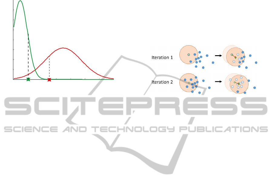
Gaussian Mixture Model
A Gaussian mixture model as introduced in (Tafaj
et al., 2012) is also available. This method is based
on the assumption that distances between subsequent
measurement points within a fixation form a Gaussian
distribution. Furthermore distances between mea-
surement points that belong to a saccade also form
a Gaussian distribution, but with different mean and
standard deviation. A maximum likelihood estima-
tion of the parameters of the Mixture of Gaussians
is performed. Afterward for each measurement point
the probability that it belongs to a fixation or to a sac-
cade can be calculated and fixation/saccade labels are
assigned based on these probabilities (Figure 2). The
major advantage of this approach is that all parame-
ters can be derived from the data. One could evaluate
data recorded during an unknown experiment with-
HEALTHINF2015-InternationalConferenceonHealthInformatics
214
out the need to specify any thresholds or experimental
conditions. The method has been evaluated in several
studies (Kasneci et al., 2014a; Kasneci et al., 2015).
Probability density
Distance between measurements
Fixations
Saccades
Figure 2: Fit of two Gaussian distributions to the large dis-
tances between subsequent measurements within saccades
and the short distances between fixations. Two sample
points are shown, one with higher probability to belong to
a fixation (left) and one with a higher probability for a sac-
cade (right).
3.3 Fixation Clustering
After identification of fixations and saccades the fix-
ations can also be clustered. Areas with a high den-
sity of fixations are likely to contain semantically rel-
evant objects. Clustering fixations either by neigh-
borhood thresholds or mean-shift clustering (as pro-
posed by (Santella and DeCarlo, 2004)) results in
data-driven, automatically assigned areas of interest.
This step reduces time consuming manual annotation
and enables data analysis without prior knowledge of
the analyst influencing the results (Figure 4).
Clusters of saccades correspond to frequent paths
taken by the eyes. Fixation and saccade clusters can
be calculated on the scan patterns of one subject or
cumulative on a group of subjects.
Standard Clustering Algorithm
This greedy algorithm requires the definition of a
minimum number of fixations that will be considered
a cluster and the maximum radius of a cluster. Fix-
ations are sorted in descending order of the number
of included gaze points. Starting with the longest
fixation, the algorithm iterates over all fixations,
checking whether they fulfill the conditions of
building a cluster with the biggest one. If the number
of found fixations is sufficient, all found fixations
are assigned to the same cluster and excluded from
further clustering. If not, the first fixation cannot be
assigned to any cluster and the algorithm starts again
from the second longest fixation.
Mean-shift Clustering
The mean-shift clustering method assumes that mea-
surements are sampled from Gaussian distributions
around the cluster centers. The algorithm converges
towards local point density maxima. The iterative
procedure is shown in Figure 3. One of the main
advantages is that it does not require the expected
number of clusters in advance but determines an
optimal clustering based on the data.
Figure 3: Simplified visualization of the mean-shift algo-
rithm for the first two iterations at one starting point. In each
iteration the mean (green square) of all data points (blue cir-
cles) within a certain window around a point (big red circle)
is calculated. In the next iteration the procedure is repeated
with the window shifted towards the previous mean. This is
done until the mean convergence.
Cumulative Clustering
The clustering algorithms mentioned above can also
be used on the cumulative data of more than one sub-
ject or more than one experiment condition. This way
cumulative population clusters can be formed. They
are more robust to noise and individual viewing be-
havior differences. The parameters of the algorithms
are adapted for cumulative usage (e.g. the number
of minimum fixations for the standard algorithm de-
pends on the number of data sets used for cumulative
analysis), but the way the methods work remain the
same.
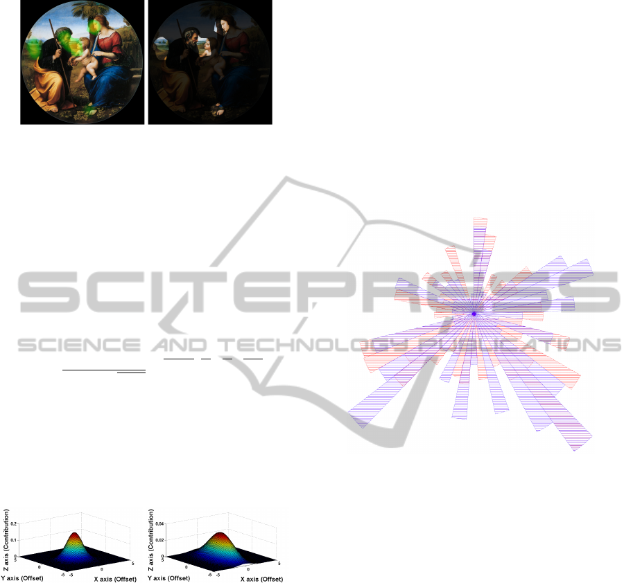
3.4 Areas of Interest (AOIs)
For the evaluation of specific regions, Eyetrace2014
provides the possibility to annotate AOIs manually or
by automatic conversion of fixation clusters. While
the automated way is comfortable, the generated
AOIs are not required to intuitively make sense. An-
notating semantically meaningful areas is still done
best by a human. Therefore we provide a graphi-
cal editor where polygonal AOIs can be defined and
edited with few mouse clicks. Figure 4 shows an ex-
ample of manually and automatically defined AOIs
and also visualizes that automatically generated AOIs
tend to - but do not necessarily - correspond to inter-
esting regions of the image. All generated AOIs can
be saved to disk and reused in other sessions or pro-
grams.
Eyetrace2014-EyetrackingDataAnalysisTool
215

Figure 4: Simultaneous overlay of multiple visualization
techniques for one scanpath of an image viewing task. The
background image is shown together with a scanpath repre-
sentation of fixed-size fixation markers (small circles) and
generated fixation clusters (bigger ellipses) for left (green)
and right (blue) eye. AOIs were annotated by hand (marked
as white overlay).
3.5 Scanpath Comparison
Various characteristics of the scanpaths such as fixa-
tion durations and saccade lengths, as well as visual
attention distribution and glance proportion towards
fixation clusters can be calculated and exported. In
addition to these global time-integrated scanpath de-
scriptors, it is also possible to automatically compare
scanpaths to each other. We therefore implemented
a variant of ScanMatch (Cristino et al., 2010) that
makes use of the fixation clusters and areas of inter-
est described above. Fixation clusters are used in or-
der to label the scanpath data (Santella and DeCarlo,
2004). ScanMatch then tries to align the fixation se-
quences by the Needleman-Wunsch string alignment
algorithm.
We are planning to extend the scanpath compari-
son capabilities with automated image segmentation
and object tracking functionality for AOI annotation
as well as probabilistic scanpath comparison metrics.
4 DATA VISUALIZATION
The software allows simultaneous visualization of
multiple scanpaths. These may represent different
subjects, subject groups or distinct experiment con-
ditions. The scan patterns are rendered in real-time
as an overlay to an image or video stimulus. Vari-
ous customizable visualization techniques are avail-
able: Fixations that encode fixation duration in their
circular size, elliptical approximations encoding spa-
tial extend as well as attention and shadow maps. Ex-
ploratory data analysis can be performed by travers-
ing through the time dimension of the scan patterns as
if it was a video. Most of the visualizations are inter-
active so that placing the cursor over the visualization
of e. g. a fixation gives access to detailed information
such as its duration and onset time.
4.1 Fixations and Fixation Clusters
The visualization of fixations and fixation clusters has
to account for their spatial and temporal information.
It is common to draw them as circles of either uniform
size or to encode the fixation duration as the circle di-
ameter. Besides these options, Eyetrace2014 offers
an ellipse fit visualization to the spatial extend of the
fixation. The eigenvectors of all measurement points
assigned to the fixation are calculated. These vectors
point into the direction of highest variance within the
data (see Figure 5). This visualization is especially
useful when evaluating fixation filters and their pa-
rameters. We found it interesting and important to see
that the jitter within a fixation does often not form a
circular, but a stretched ellipse.
Figure 5: The two eigenvectors of Gaussian distributed
samples (that correspond to the directions of highest vari-
ance). These are used as the major and minor axes for an
elliptic fit.
4.2 Attention and Shadow Maps
Attention maps are one of the most common eye-
tracking analysis tools, besides the high number of
subjects that have to be measured in order to get reli-
able results (Pernice and Nielsen, 2009). In order to
enable fast attention map rendering even for a large
number of recordings and high resolution, the atten-
tion map calculation utilizes multiple processor cores.
Attention maps can be calculated for gaze points, fix-
ations and fixation clusters. We provide the classical
red-green color palette for attention maps as well as
blue version for color-blind persons.
For the gaze point attention map each gaze point
contributes as a two dimensional Gaussian distribu-
tion. The final attention map is then the sum over
HEALTHINF2015-InternationalConferenceonHealthInformatics
216
(a) (b)
Figure 6: An attention map calculated for fixation clusters
(a) and the corresponding shadow map (b).
all Gaussians. The Gaussian distribution is specified
by the two parameters size and intensity which are
adjustable by the user. This Gaussian distribution is
circular because gaze points do not have information
about orientation and size. For fixations and fixation
clusters the elliptic fit is used to determine the shape
and orientation of the Gaussian distribution. Figure 7
shows an example of a circular Gaussian distribution
(a) and a stretched, elliptical one (b).
P(x, y) =
1
σ
1
σ
2
2π
√
1 −ρ
e
−
1
2(1−ρ
2
)
(
x
2
σ
2
1
+
y
2
σ
2
2
−
2ρxy
σ
1
σ
2
)
(1)
Equation 1 shows the Gaussian distribution in the
two dimensional case. σ
1
and σ
2
are the variance in
horizontal and vertical direction respectively (see Fig-
ure 7). x and y are the offsets to the center of the
Gaussian distribution (see Figure 7). The correlation
coefficient ρ is zero in Figure 7 to simplify the case.
(a) (b)
Figure 7: Two Gaussian distribution calculated with σ
1
=
σ
2
= 1 (a) and σ
1
= 1 and σ
2
= 5 (b).
A variant of the attention map is the shadow map
that reveals only areas that were looked at (see Fig-
ure 6(b)). Its calculation is identical to that of the at-
tention map with the difference of a smoothing step
in order to show the border regions with higher sen-
sitivity. This is done by calculating the n-th root of
each map value where n is a user-defined parameter
that regulates the desired smoothing.
4.3 Saccades
Saccades are typically visualized as arrows or lines
connecting two fixations.
Besides this, a statistical evaluation can be visu-
alized as a diagram called anglestar. It consists of a
number of slices and a rotation offset. A slice of the
anglestar codes in its length the number of saccades
with the same angular orientation as the slice (e.g. if
the slice represents the angles between 0
◦
and 45
◦
the
number of saccades within that angle range contribute
to that slice) to the horizontal axis is considered. The
extend of a slice from the center of the star can repre-
sent the quantity, summed length or summed duration
of the saccades towards that direction. Figure 8 shows
a diagram where the extension of the slices is based
on the summed length of the saccades.
Figure 8: Representation of an anglestar, the red part repre-
sents data of the left eye, the blue part refers to data of the
right eye.
4.4 AOI Transitions Diagram
For some evaluation cases it is interesting in which
sequence attention is shifted between different areas.
The AOI transitions diagram (Fig. 9) visualizes the
transition probabilities between AOIs during a spe-
cific time period. The color of the transition is in-
herited from the AOI with most outgoing saccades.
Hovering the mouse over an AOI shows all transitions
from this AOI and hides the transitions from all other
AOIs. Hovering the cursor over a specific transition
displays an information box containing the number of
transitions in both directions. Figure 9(b) e.g. shows
that after watching AOI cluster3 in more than 80%
of cases gaze stayed at cluster3, in some cases gaze
moved on towards cluster1 or cluster2 and in very few
cases towards cluster4 and cluster5.
Eyetrace2014-EyetrackingDataAnalysisTool
217

(a) (b)
Figure 9: Diagram of the transitions between AOIs. The
graphic is interactive and can blend out irrelevant edges if
one AOI is selected (b).
5 DATA EXPORT
5.1 Statistics
General Statistics
Independent of all other calculations it is possible to
calculate some general gaze statistics. These include
the horizontal and vertical gaze activity, minimum,
maximum and average speed of the gaze. These
statistics shine a light on the agility and exploratory
behavior of the subjects and can be exported in a
format ready to use in statistical programs such as
JMP or SPSS.
AOI Statistics
Numerous gaze characteristics can be calculated for
AOIs, such as the total number of glances towards the
AOI, the time of the first glance, glance frequency, to-
tal glance time, the glance proportion towards the AOI
in respect to the whole recording and the minimum,
maximum and mean glance duration. These statistics
are a supplement to the AOI transitions diagram and
can also be exported.
5.2 Visualization
The transition diagram as well as every visualization
can be exported either loss-less as vector graphics or
as bitmaps (png, jpg). Eyetrace2014 provides the op-
tion to export the information about the subject (e.g.
age, dominant eye) and the parameters used for cal-
culation and visualization as a footer in the exported
image. That way results can be reproduced and un-
derstood based solely on the exported image.
5.3 Evaluation Results
After calculating fixations, fixation clusters or cumu-
lative clusters Eyetrace2014 provides the possibility
to export them as a text file.
Fixations are exported in a table including the run-
ning number, the number of included points, x and y
coordinate, radius and if calculated the id of the clus-
ter this fixation belongs to. The text file for the clus-
ters and cumulative clusters include an ID number,
the number of fixations contained, mean x, mean y
and the radius.
Besides the already mentioned text files, fixations
saccades and measurement error sections can be ex-
ported in order to allow extensive further processing
in statistics programs, choosing the export option ”ex-
port events”.
6 CONCLUSION AND OUTLOOK
Summarizing our work of the last year and a half we
believe that Eyetrace2014 is a well structured pro-
gram, advantageous enough to use it for university
research but with its convenient handling nonetheless
usable for persons without broad eye tracking expe-
rience, e.g. for teaching students. The major advan-
tages of the software are the flexibility of algorithms
and their parameters as well as their actuality in re-
spect to the state of the art.
Eyetrace2014 has already been employed in sev-
eral research projects, ranging from the viewing of
fine art recorded via a static binocular SMI infrared
eye-tracker to on-road and simulator driving experi-
ments (Kasneci et al., 2014b; Tafaj et al., 2013) and
supermarket search tasks (Sippel et al., 2014; Kasneci
et al., 2014c) recorded via a mobile Ergoneers Dikab-
lis tracker.
Nevertheless there are many plans to extend the
Eyetrace software bundle in the next versions.
Besides the mandatory implementation of new
eye tracker models to EyetraceButler we will extend
the quality-check possibilities for the EyetraceButler
plug-ins.
We want to extend the general and AOI based
statistics calculations, add new calculation or visual-
ization algorithms and make the existing ones more
interactive and transparent. A special focus will be
given the analysis and processing of saccadic eye
movements as well as to the automated annotation of
AOIs for dynamic scenarios (K
¨
ubler et al., 2014) and
non-elliptical AOIs.
We plan on including further automated scanpath
comparison metrics, such as MultiMatch (Dewhurst
et al., 2012) or SubsMatch (K
¨
ubler et al., 2014).
Another relevant area is the monitoring of vigi-
lance and workload during the experiment. Especially
for medical applications such as reaction or stimu-
HEALTHINF2015-InternationalConferenceonHealthInformatics
218

lus sensitivity testing the mental state of the subject
is of importance. Available data such as the pupil
dilation, fatigue waves (Henson and Emuh, 2010),
saccade length differences (Di Stasi et al., 2014) and
blink rate may give important insight into the data and
even yield e.g. cognitive workload weighted attention
maps.
ACKNOWLEDGEMENTS
We want to thank the department of art history at
the university of Vienna, especially Johanna Aufreiter
and Caroline Fuchs for the inspiring collaboration.
The project was partly financed by the the WWTF
(Project CS11-023 to Helmut Leder and Raphael
Rosenberg).
REFERENCES
Blignaut, P. (2009). Fixation identification: The optimum
threshold for a dispersion algorithm. Attention, Per-
ception, & Psychophysics, 71(4):881–895.
Brinkmann, H., Commare, L., Leder, H., and Rosenberg, R.
(2014). Abstract art as a universal language?
Cristino, F., Math
ˆ
ot, S., Theeuwes, J., and Gilchrist, I. D.
(2010). ScanMatch: a novel method for compar-
ing fixation sequences. Behavior research methods,
42(3):692–700.
Di Stasi, L. L., McCamy, M. B., Macknik, S. L., Mankin,
J. a., Hooft, N., Catena, A., and Martinez-Conde, S.
(2014). Saccadic eye movement metrics reflect surgi-
cal residents’ fatigue. Annals of surgery, 259(4):824–
9.
Henson, D. B. and Emuh, T. (2010). Monitoring vigilance
during perimetry by using pupillography. Investiga-
tive ophthalmology & visual science, 51(7):3540–3.
Kasneci, E., Kasneci, G., K
¨
ubler, T. C., and Rosenstiel, W.
(2014a). The applicability of probabilistic methods
to the online recognition of fixations and saccades in
dynamic scenes. In Proceedings of the Symposium on
Eye Tracking Research and Applications, pages 323–
326. ACM.
Kasneci, E., Kasneci, G., K
¨
ubler, T. C., and Rosenstiel, W.
(2015). Online recognition of fixations, saccades, and
smooth pursuits for automated analysis of traffic haz-
ard perception. In Artificial Neural Networks, pages
411–434. Springer.
Kasneci, E., Sippel, K., Aehling, K., Heister, M., Rosen-
stiel, W., Schiefer, U., and Papageorgiou, E. (2014b).
Driving with binocular visual field loss? a study on
a supervised on-road parcours with simultaneous eye
and head tracking. PloS one, 9(2):e87470.
Kasneci, E., Sippel, K., Aehling, K., Heister, M., Rosen-
stiel, W., Schiefer, U., and Papageorgiou, E. (2014c).
Homonymous visual field loss and its impact on vi-
sual exploration - a supermarket study. Translational
Vision Science and Technology, In Press.
Klein, C., Betz, J., Hirschbuehl, M., Fuchs, C., Schmiedtov,
B., Engelbrecht, M., Mueller-Paul, J., and Rosenberg,
R. (2014). Describing art? an interdisciplinary ap-
proach to the effects of speaking on gaze movements
during the beholding of paintings.
K
¨
ubler, T. C., Bukenberger, D. R., Ungewiss, J., W
¨
orner,
A., Rothe, C., Schiefer, U., Rosenstiel, W., and Kas-
neci, E. (2014). Towards automated comparison of
eye-tracking recordings in dynamic scenes. In EUVIP
2014.
Pernice, K. and Nielsen, J. (2009). How to conduct eye-
tracking studies. Nielsen Norman Group.
Rosenberg, R. (2014). Blicke messen. vorschl
¨
age f
¨
ur
eine empirische bildwissenschaft. Jahrbuch der Bay-
erischen Akademie der Sch
¨
onen K
¨
unste, 27:71–86.
Salvucci, D. D. and Goldberg, J. H. (2000). Identifying
fixations and saccades in eye-tracking protocols. In
Proceedings of the 2000 symposium on Eye tracking
research & applications, pages 71–78. ACM.
Santella, A. and DeCarlo, D. (2004). Robust clustering of
eye movement recordings for quantification of visual
interest. Proceedings of the Eye tracking research &
applications symposium on Eye tracking research &
applications - ETRA’2004, pages 27–34.
Sippel, K., Kasneci, E., Aehling, K., Heister, M., Rosen-
stiel, W., Schiefer, U., and Papageorgiou, E. (2014).
Binocular glaucomatous visual field loss and its im-
pact on visual exploration-a supermarket study. PloS
one, 9(8):e106089.
Tafaj, E., Kasneci, G., Rosenstiel, W., and Bogdan, M.
(2012). Bayesian online clustering of eye movement
data. In Proceedings of the Symposium on Eye Track-
ing Research and Applications, pages 285–288. ACM.
Tafaj, E., K
¨
ubler, T. C., Kasneci, G., Rosenstiel, W., and
Bogdan, M. (2013). Online classification of eye track-
ing data for automated analysis of traffic hazard per-
ception. In Artificial Neural Networks and Machine
Learning–ICANN 2013, pages 442–450. Springer.
Tafaj, E., K
¨
ubler, T. C., Peter, J., Rosenstiel, W., Bogdan,
M., and Schiefer, U. (2011). Vishnoo: An open-
source software for vision research. In Computer-
Based Medical Systems (CBMS), 2011 24th Interna-
tional Symposium on, pages 1–6. IEEE.
Eyetrace2014-EyetrackingDataAnalysisTool
219
