ROBE

Knitting a Tight Hub for Shortest Path Discovery in Large Social Graphs

Lixin Fu and Jing Deng

Department of Computer Science, University of North Carolina at Greensboro, Greensboro, NC 27412, U.S.A.

Keywords: Shortest Paths, Error Rate, Social Networks.

Abstract: Scalable and efficient algorithms are needed to compute shortest paths between any pair of vertices in large

social graphs. In this work, we propose a novel ROBE scheme to estimate the shortest distances. ROBE is

based on a hub serving as the skeleton of the large graph. In order to stretch the hub into every corner in the

network, we first choose representative nodes with highest degrees that are at least two hops away from

each other. Then bridge nodes are selected to connect the representative nodes. Extension nodes are also

added to the hub to ensure that the originally connected parts in the large graph are not separated in the hub

graph. To improve performance, we compress the hub through chain collapsing, tentacle retracting, and

clique compression techniques. A query evaluation algorithm based on the compressed hub is given. We

compare our approach with other state-of-the-art techniques and evaluate their performance with respect to

miss rate, error rate, as well as construction time through extensive simulations. ROBE is demonstrated to

be two orders faster and has more accurate estimations than two recent algorithms, allowing it to scale very

well in large social graphs.

1 INTRODUCTION

As part of “big data” analytics, finding the shortest

paths in large social networks has been an intense

research area in both academia and industry. The

shortest-path query is a classic problem in graph

theory. Breadth-First Search (BFS) can be used on

unweighted graphs, such as those in Facebook.com,

with an O(V+E) computational complexity, where V

and E are the numbers of vertices and edges of the

graph, respectively. Due to the sheer sizes of the

large social graphs, the algorithm cannot be directly

applied. Instead, scalable and efficient algorithms

must be developed.

In order to address shortest-path queries with

scalable and distributed solutions, researchers rely

on different types of techniques. For instance, a

highway transportation system approach is used in

(Cohen, Halperin et al. 2003). Instead of using

global landmarks as some shortest path algorithms

do, we use a much smaller graph that is applicable

with BFS. In this work, we propose a new hub-based

algorithm called ROBE (Representative nodes

Ornamented by Bridge nodes and Extension nodes).

Our main contributions in this work are:

1. We propose a new hub concept and

construction scheme, and give several results that

guarantee the representativeness and connectivity.

2. We propose new hub compression strategies to

reduce the number of nodes in the hub while still

maintaining the accuracy of shortest path queries.

3. We design a query computation algorithm on

the compressed hub and conduct extensive

simulations to confirm the advantages of our new

algorithms.

The rest of the paper is organized as follows.

Section 2 surveys related work in the field and

distinguishes our approach from others. Sections 3

and 4 provide detailed description of our hub

construction and hub compression techniques,

respectively. Query evaluation is presented in

Section 5, followed by performance evaluation on

different data sets in Section 6. In Section 7, we

conclude the work.

2 RELATED WORK

Shortest-path discovery is a classic problem in

computer science. For an extensive related work

discussion, the readers are referred to for instance

Fu L. and Deng J..

ROBE - Knitting a Tight Hub for Shortest Path Discovery in Large Social Graphs.

DOI: 10.5220/0005353500970107

In Proceedings of the 17th International Conference on Enterprise Information Systems (ICEIS-2015), pages 97-107

ISBN: 978-989-758-096-3

 2015 SCITEPRESS (Science and Technology Publications, Lda.)

(Wei 2011), a state-of-the-art work in the field. We

discuss some of the latest developments in the field

in the following.

Traditional approaches to the shortest-path

discovery problem (Dijkstra 1959) (Bellman 1958),

while elegant and accurate by design, do not scale to

the large social networks today. The main issue is

the large number of vertices and edges: they

introduce significant delays on I/O storage and

memory access. Another unique property of social

networks is the small degree of separation, which

states that any two vertices are likely to be

connected through some paths with hop-counts no

more than four (Backstrom, Boldi et al. 2012).

Considering these computational costs and the

unique properties of large social networks,

researchers proposed various techniques to improve

the scalability and efficiency of the shortest-path

discovery algorithms. For instance, in (Potamias,

Bonchi et al. 2009), Potamias et al. proposed a

landmark-based distance indexing technique. The

landmarks are supposed to represent different

regions. Then the distances among themselves are

computed. Shortest-distance queries are estimated

by distances of the two nodes to the landmarks. Such

an approximation technique based on triangulation

has been used by different researchers, for example,

the 3-hop scheme (Jin, Xiang et al. 2009), the TEDI

scheme based on tree decomposition (Wei 2011), the

query-dependent local landmark scheme (Qiao,

Cheng et al. 2012), and the highway-centric scheme

(Jin, Ruan et al. 2012).

Zhao et al. (Zhao, Sala et al. 2010) mapped

nodes in high dimensional graphs to positions at a

low dimensional Euclidean space in a scheme called

Orion. To improve non-landmark coordinate

calculation in Orion, a new algorithm called Pomelo

(Chen, Chen et al. 2011) is proposed to calculate the

graph coordinates in a decentralized manner. Gao et

al. provides relational approach to process shortest

queries in graph (Gao, Jin et al. 2011).

Akiba et al. (Akiba, Iwata et al. 2013) claim that

BFS on every vertex using pruning and simultaneous

searches with bitwise operations can process exact

distance queries efficiently. They experiment large

graphs with hundreds of millions of edges. Through

walking consecutive gate nodes in a gate graph, a

new approach of graph simplification can cover non-

local nodes while preserving distances (Ruan, Jin et

al. 2011).

Feder and Motwani researched on graph

compression through cliques (Feder and Motwani

1995). It is well known that the problem of whether

there is a clique of size k in a given graph is NP-

hard. In this work, we design a clique detection

algorithm similar to the famous association rule

mining algorithm Apriori (Agrawal and Srikant

1994). The clique compression is especially

important in social networks because cliques are

quite common in such graphs. For general graph

queries, a smaller graph is computed to preserve the

original query in a compression framework proposed

by Fan et al. (Fan, Li et al. 2012). Other work related

to graph compression includes (Karande, Chellapilla

et al. 2009, Apostolico and Drovandi 2009).

For approximate distance oracles, Thorup and

Zwick gave an algorithm (Thorup and Zwick 2005)

that pre-computes a data structure of size O(kn

1+1/k

)

in O(kmn

1/k

) and answers a distance query

approximately in O(k) time, where m is the number

of edges, n is the number of nodes, and k is a certain

constant. The query is approximate, but no more

than a factor of 2k-1 of the true distance away. On

top of this, Baswana and Sen further improved the

expected construction times of the approximate

oracles to O(n

) (Baswana and Sen 2006).

Recently, Gubichev et. al proposed a sketch-

based index to compute distance queries together

their corresponding paths (Gubichev, Bedathur et al.

2010). Another sketch-based algorithm given by

Sarma et. al computes the distance queries for web-

scale large graphs (Sarma, Gollapudi et al. 2010). It

estimates the distance through the sketches of the

source node and the destination node.

3 HUB CONSTRUCTION

3.1 Goals of Hub Construction

Essentially, our idea is to build a “robe” – the hub

graph and pre-compute pairwise shortest distances

between all the hub nodes. A “query miss” happens

when the hub is not a connected graph though they

are originally connected in the input graph. A good

hub should satisfy the following properties:

 Good representation so that the missing rate is

low or even zero;

 Good connection among the nodes inside the

hub so that their shortest distances are close to

the actual shortest distance in the original

graph G;

 Low construction time. This is needed so that

the overhead of constructing the hub is as low

as possible.

ICEIS2015-17thInternationalConferenceonEnterpriseInformationSystems

3.2 Representative Nodes, RN

We first sort all the nodes by degrees in decreasing

order and choose the nodes one by one starting from

the node with highest degree, such that the newly

chosen one must not be a direct neighbour of any

existing members in the set. The restriction is to

leave chances to nodes in sparser regions so that the

hub is spread wide. These nodes are termed

representative nodes (the set is RN). The graph is

called G

, with |RN| singleton nodes.

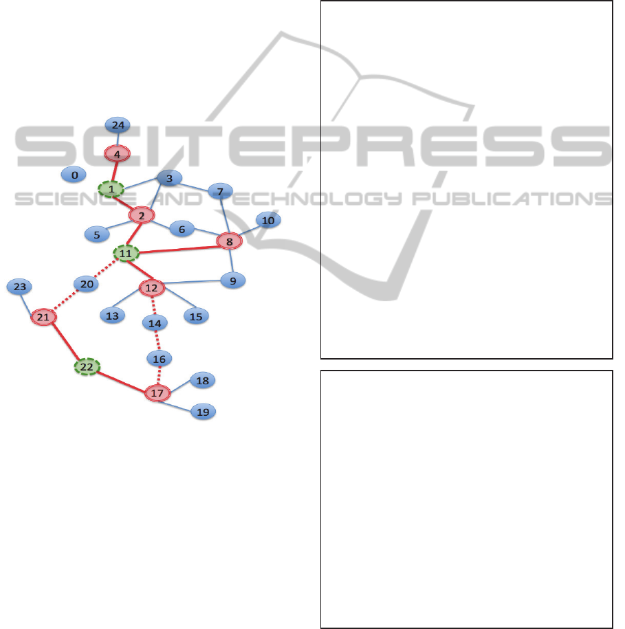
In Figure 1, for instance, nodes 2, 8, 12, 17, 21,

and 4 will be chosen as the representative nodes.

Despite that node 11 has a large node degree (of 4),

it is not qualified to serve because its neighbours 2

and 8 have already been chosen.

Figure 1: Illustration of rn, bn, and en in a graph. Double-

ovals (in red) are representative nodes. Dashed-ovals (in

green) are bridge nodes. Dotted-ovals (in darker blue) are

extension nodes. The thick solid lines (in red) represent

bridge edges. The dotted lines (in red) represent extension

edges.

THEOREM 1. (ZERO MISS RATE) If the input graph is

connected and the above RN selection algorithm is

applied, any node in the graph will always have at

least one representative node within distance of two.

That is, the miss rate will be zero if the hub is

eventually connected and two-hop neighbors of the

hub nodes are searched.

ROOF: we prove it by contradiction. Suppose

there is a node u and the closest representative node

U is at least 3-hops away: u - y - x - U. Then there

exists at least one neighbor, node y, in node u’s

neighbor set, that does not have a representative

node within one hop (otherwise node u can choose

such a neighbor toward a representative node for

two hops). Based on our representative node

selection rule, node y would have been chosen as a

representative node. Node u’s distance to the closest

representative node is then 1, which contradicts to

our assumption that the closest representative is at

least 3-hop away.

The detailed algorithm of selecting representative

nodes is described in Algorithm 3.1. The intersection

in line 3 and 4 takes linear time O(|RN| +D), where

D is the max degree of input graph G. Line 4 takes

Algorithm 3.2: Selection of

Bridge Nodes

Input: input graph linked lists

ig, G

Output: a set of bridge nodes

1. Sort lists in G\G

decreasing order of degrees

2. for each node i

3. if (node i does not

connect at least two RN nodes)

continue

4. if ( it does not add

connectivity of G

) continue

5. add i into BN and update

the distance between two RN

odes it connects to 2.

Algorithm 3.1: Selection of

Representative Nodes

Input: input graph linked lists

Output: a set of representative

nodes

1. Sort the lists in decreasing

order according to degrees

2. RN = {v

}, v

is the node ID

of the first list

3. for each next ID Vi, see if

’s neighbors are in RN

4. if not, i.e. ig[v

] ∩ RN =

φ, insert it in RN in right

position using binary search so

that RN is still sorted. This

step is similar to insertion

sort.

5. if yes, continue to node ID

of next list

6. repeat step 3-5 until the

lists are all examined.

ROBE-KnittingaTightHubforShortestPathDiscoveryinLargeSocialGraphs

O(log|RN|+|RN|). Time complexity for Algorithm

3.1 is then O(|RN|

). Typically, D is smaller than

|RN| for large graphs. The bridge node selection

algorithm is presented in Algorithm 3.2.

3.3 Bridge Nodes, BN

Since G

only contains totally isolated singleton

nodes, we need to add other non-representative

nodes, in decreasing order of degrees if they can

directly connect at least two representative nodes

and improve the connectivity of G

. We call these

connecting nodes as bridge nodes. The graph

composed of representative nodes, bridge nodes, and

their edges is called G

. In Figure 1, for example,

nodes 11, 1, and 22 are chosen as bridges in order.

3.4 Extension Nodes, EN

Even though the bridge nodes greatly improve

connectivity of G

, the graph G

may still be

disconnected. For example, in Figure 1, the

component of nodes 17, 22, and 21 is separated from

the other larger component with six nodes. To

address this problem, we select additional nodes to

connect the isolated components in G

The newly selected nodes are called extension

nodes, en, and the edges that connect the

disconnected components are called extension edges.

The graph that extends G

with extension nodes and

edges is called G

– the “robe” we use to estimate

shortest paths. In this paper, we also call G

as hub

graph (HG). In Figure 1, nodes 14, 16, and 20 are

extension nodes and the extension edges are shown

in dotted lines.

Algorithm 3.3 shows the details of finding the

extension nodes and adding them with extension

edges to graph G

. The first two lines analyze the

component structures of input graph G and G

BFS calls, through which we can find the component

sizes and check whether any two nodes are from the

same connected component.

Lines 4 through 8 explore and add pairwise,

component-to-component connections in G

if they

are from the same component in G. H

and H

are the

smallest node IDs as representatives in components i

and j respectively while num_comp is the total

number of components in G

. The BFS calls in line

7 in Algorithm 3.3 are partial searches: only to the

third iterations at most in order to reach their target

nodes T (e.g. nodes 12 and 11 in Figure 1). In the

following theoretic analysis, we find that the lengths

of the extension paths will be two or three. Lastly, in

order to improve performance we start with smallest

components (in line 3).

HEOREM 2. (DISTANCE OF THREE) Suppose nodes u

and v are two closest representative nodes in

different components of G

and are connected in G,

then |u-v| = 3 in G.

ROOF:

1) The distance cannot be one because they cannot

be direct neighbors according to our representative

selection rule.

2) The distance cannot be two. If u-x-v, then x must

be a bridge node because it connects two

representative nodes u and v. Then u and v would be

in the same component, a contradiction to our

assumption.

3) The distance cannot be four or more if they are

connected in G. Suppose the path is u-u1-x-v1-v,

then the node x should be chosen as a representative

node as well thus forcing u and v to be connected in

. In our example, u and v are nodes 17 and 12.

4 HUB COMPRESSION

4.1 Rationale of Hub Compression

The hub containing representative nodes, bridge

nodes, and extension nodes can be quite large.

Experiments show that vast majority of the time of

Algorithm 3.3: Selection of

Extension Nodes

Input: input graph linked lists

G, G

Output: a set of extension nodes

1. BFS(G) to find connected

components in G

2. BFS(G

) to find all connected

components in G

3. sort components of G

increasing sizes

4. for (int i=0; i<num_comp;

i++)

5. for (int j=i+1;

j<num_comp; j++)

6. if ( H

and H

are connected

in G)

7. BFS(H

) to 3rd generation

to meet a node T in

component j

8. add extension nodes and

edges between H

and T to G

ICEIS2015-17thInternationalConferenceonEnterpriseInformationSystems

100

hub construction is on the writing of the pre-

computed pair-wise distances between hub nodes to

disks. This motivates us to reduce the number of

nodes in the hub so that distance computation can

still be performed without storing all of them on

disk.

4.2 Retracting the Tentacles and

Collapsing the Chains

The first method of compression is to remove the

nodes with a degree of one or two. The leaves that

grow out of nodes called home nodes. The nodes

with degree two are called chain nodes. From any

chain node, we can search from both sides until the

both ends have a degree other than two. We can

choose the closer end as its home node. If only one

end is a leaf, then this chain is called a tentacle. The

other end of the tentacle will be the home node for

all the nodes on the tentacle. If neither end is a leaf,

this chain will be an inside chain. The algorithm to

retract the tentacles, leaves, and to remove chain

nodes is called collapse (see Algorithm 4.1).

Two maps, leaf_map and chain_map, are used to

store the home nodes of the leaf nodes and chain

nodes. In Figure 1, the home nodes are 1 and 11 for

two leaves 4 and 8 respectively (saved in leaf_map

in line 3 of Algorithm 4.1). The long ring chain 11-

12-14-16-17-22-21-20-11 will be saved in

chain_map in line 7 with node 11 being the home of

the chain. Another chain 4-1-2-11 is a tentacle since

one end is a leaf (node 4). The home node is 11 for

chain nodes 1 and 2. After collapsing, the

compressed hub only has one node 11.

4.3 Compressing the Cliques

Another powerful compression technique is to

replace complete sub-graphs called cliques with so-

called super nodes. We are only interested in cliques

of size three (also called triangulation) or more. We

can choose the node with largest degree as the home

node of other super members in the same super

node. The super members are saved in super_map.

Algorithm 4.2 describes the process of finding

cliques and super nodes. It is similar to a standard

association rule mining algorithm called Apriori. We

will use an example shown in Figure 2 to illustrate.

First, we scan the linked lists and remove the nodes

with degree zero or one. Also we only retain the list

nodes with larger IDs than the node ID. For the first

list 1: 2, 3, 4, 7, 13, 14, we self join clique L

= {

{1,2}, {1,3}, {1,4}, {1, 7}, {1, 13}, {1, 14}} and

create candidates C

= { {1, 2, 3}, {1, 2, 4}, {1, 2,

7}, {1, 2, 13}, {1, 2, 14}, {1, 3, 4}, {1, 3, 7}, {1, 3,

13}, {1, 3, 14}, {1, 4, 7}, {1, 4, 13}, {1, 4, 14}, {1,

7, 13}, {1, 7, 14}, {1, 13, 14}} (Line 4 in Algorithm

4.2).

Similar to Apriori algorithm, the join of two

clique sets of size k {N

, N

, ...N

k-1

, N

} and {N

, ...N

k-1

, N

k+1

} that have first k-1 common nodes

generates a candidate set {N

, N

, ...N

k-1

, N

k+1

If there is an edge from N

to N

k+1

(by examining

Algorithm 4.2: Compress Cliques

Input: G

Output: super_map

1. remove nodes with degree 1 or

below

2. only retain nodes with higher

IDs

3. for each non-empty list

// generate candidate cliques

4. candidate C

= L

i-1

self

join L

i-1

5. check if they have the

joining edge to grow to L

6. repeat steps 4 and 5

until there is no more growth

7. save the largest L

candidate clique list

8. sort the candidate list in

decreasing sizes

9. choose the top one and save

it in super_map

10. remove it and any clique

that intersects with it

11. repeat 9 and 10 until the

candidate list is empty

12. choose the node with largest

degree as the home node of other

members in the same clique

Algorithm 4.1: Collapse

Input: G

Output: leaf_map, and chain_map

1. for each linked list in G

2. if (list size is one)

3. leaf_map.put(leaf_ID,

home_ID)

4. if (list size is two)

5. expand from node i left to

get left chain and left_home

6. expand to right to get right

chain and right_home

7. form a chain and save it in

chain_map

ROBE-KnittingaTightHubforShortestPathDiscoveryinLargeSocialGraphs

101

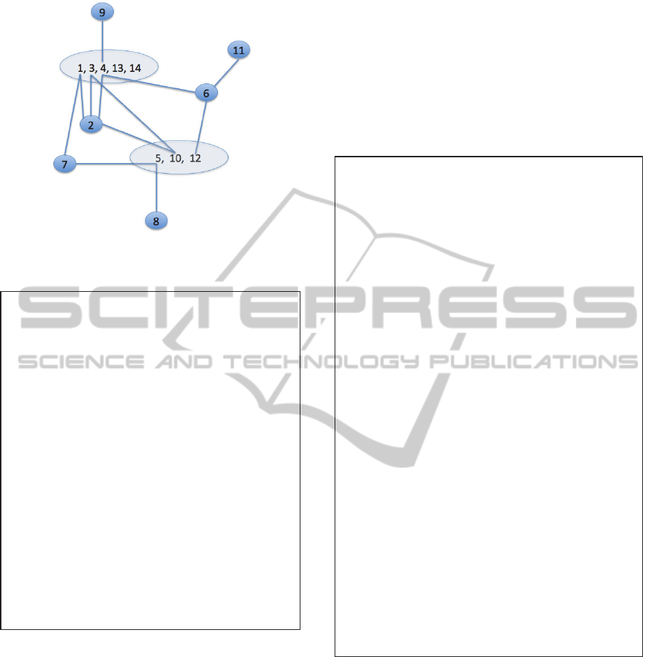
Figure 2: Illustration of an input graph with two cliques,

one with 5 nodes and the other with 3 nodes.

's adjacency list), the new candidate will be a

newly grown clique of size k+1. Otherwise, it will

be eliminated from the candidate list C

k+1

(indicated

by stricken crossed lines above). Since the joining

edge (2, 7) does not exist, {1,2,7} will not be a

clique of size 3. The remaining is L

. Self join L

we have C

= {{1, 2, 3, 4}, {1, 3, 4, 13}, {1, 3, 4,

14}, {1, 4, 13, 14}}. L

= C

. C

= {{1, 3, 4, 13, 14}

= L

. Finally, we have a clique of size 5 {1, 3, 4, 13,

14} and add it in the candidate clique list.

To reduce the query evaluation complexity, we

require that the cliques are disjoint. Using a greedy

strategy, we choose the largest clique and eliminate

any candidate that overlaps with it (lines 8-11). The

final clique set is {{1, 3, 4, 13, 14}, {5, 10, 12}}.

Once the cliques are found, we then compute the

pair-wise distances among the hub nodes through

BFS and save them in a file for query evaluation.

The hub nodes hn will be the remaining nodes after

removing leaves, tentacle nodes, chain nodes, and

super members in cliques (lines 1 and 2 in

Algorithm 4.3. The pair-wise distances are

computed and stored in lines 4 through 6. Now, we

are ready to evaluate shortest distance queries.

5 QUERY EVALUATION

Since in social media graphs most nodes are of a

distance four or less (Small World Theory), we first

directly compute the shortest distance of u and v in a

given query by intersecting the neighbor set (N

) or

neighbor-of-neighbor set (N

) of u and v. This is an

accurate computation if the intersection set is non-

empty. If the shortest distance between u and v is

more than four, we will always be able to find two

nodes U and V in the hub G

within N

or N

of u

and v according to Theorem 1. One or both u and v

Algorithm 5.1: Distance (u, v)

Input: any two nodes u and v in G

Output: the shortest distance (or

estimate) between u and v.

1. if ( u = v) return 0;

2. if ( distance between u and v

is smaller than five)directly

compute by intersection and

return

3. extra =0

4. if (u is in G

) U = u;

5. else if ( N

(u) ∩ V(G

) is non

empty)

6. U is the common element;

extra++;

7. else if ( N

(u) ∩ V(G

) is non

empty)

8. U is the common element;

extra = extra +2;

9. if (v is in G

) V = v;

10.else if ( N

(v) ∩ V(G

) is non

empty)

11. V is the common element;

extra++;

12. else if ( N

(v) ∩ V(G

) is non

empty)

13. V is the common element;

extra = extra +2;

14. return extra + hub_distance

(U, V)

Algorithm 4.3: Compute Distances

Among Hub Nodes

Input: G

, leaf_map, chain_map,

super_map

Output: hub-nodes,

dist_matrix(hub_nodes)

1. remove leaf nodes, tentacle

nodes, and chain nodes from G

2. remove super members from G

the remaining nodes are hub

nodes hn

3. clean super member's lists sl

so that it only contain hub

nodes

4. for each node i in hn

5. call BFS(i) to compute the

shortest distances from i to

any other hub nodes

6. store pair-wise distances of

hub nodes in file

ICEIS2015-17thInternationalConferenceonEnterpriseInformationSystems

102

may be one of those nodes in G

We use an extra value to indicate the distance

between u and U or between v and V. If u is in G

the extra distance is zero; if N

(u) intersects with

V(G

) then extra =1; if N

(u) intersects with V(G

extra = 2. Similarly, we can set extra values for v as

well (see Algorithm 5.1).

To compute the distance between U and V in G

called hub_distance(U, V) (Algorithm 5.2), we need

to handle the cases of leaves, tentacles, chain nodes,

and super members all of which do not appear in

hub nodes. We can retrieve through a file the

distances between any two hub nodes and use extra

values (initially set to zero) as additional distance

overhead. Lines 2-3 handle the leaf cases. Hu and

Hv are the home nodes of leaves u and v, retrieved

from leaf_map. Due to the symmetry, we only show

the code for U. The code for V is similar. Lines 4-7

handles the tentacle case while lines 8-11 for self

chains. If U and V are in the same chain (lines 12-

13), the shortest distance will be the shorter one of

the path between u and v or the path through the two

homes of hub nodes. Suppose iu

and iu

are the

distances from u to two homes home1 and home2

respectively. The same for iv

and iv

. Lines 14-16

tackle the case of inside chain of two different home

nodes.

Algorithm 5.3 computes the distances hub_dist(Hu,

Hv) and handle the case of super members. If Hu

and Hv are in the same super node, their distance

will be one. If both Hu and Hv are hub nodes, we

directly retrieve the distance between them through

pre-computed, pre-stored file. The rest of lines

handles the case where one or both of Hu and Hv are

super members. For example, if Hu is a super

member, remember sl(Hu) is the neighbors of Hu

that are hub nodes. If Hv is also a super member,

then hub_dist(Hu, Hv) is the minimum distance of

all pair-wise distances between sl(Hu) and sl(Hv)

(lines 8-12)

Algorithm 5.3: Hub

dist(Hu, Hv)

Input: two nodes in G

but not

of degree one or two

Output: the distance between

them

1. if (Hu = Hv) return 0

2. if (Hu and Hv are from the

same super node)

3. return 1

4. if (both Hu and Hv are hub

nodes)

5. directly retrieve their

distance from file and return

6. if ( Hu is a super member)

extra++;

// one hop away to hub node

7. if ( Hv is a super member)

extra++;

8. min = Infinity

9. for each i in sl[Hu]

10. for each j in sl[Hv]

11. if (the retrieved

distance d from i to j <min)

12. min = d;

13. return extra + min;

Algorithm 5.2: Hub

distance(U,

Input: two nodes U and V in G

leaf_map, chain_map, super_map

Output: shortest distance

between them

1. if (U = V ) return 0;

// leaves

2. if ( U is a leaf)

3. Hu is the home node of

u; extra++;

// tentacles

4. if (U is in a tentacle)

5. Hu is home node of u;

6. iu is the distance

between u and Hu

7. extra = extra +iu

// self chain, ring

8. if ( U is in a self chain)

9. Hu is the home node

10. iu is the shorter distance

from u to Hu

11. extra = extra +iu

// U and V are in the same chain

// home1 - - U- - V - - home2

// | <-- iu

-->| <-- iu

-->|

12. if ( U and V are in the same

chain)

13. return min( iv

-iu

hub_dist(home1, home2)+ iu

+iv

)

// inside chain

14. if ( U is in an inside chain

of different ends)

15. Suppose Hu1 and Hu2 are the

ends

16. return the shortest

distance of U and V through

Hu1, Hu2, Hv1, Hv2

17. return extra + hub_dist(Hu,

Hv)

ROBE-KnittingaTightHubforShortestPathDiscoveryinLargeSocialGraphs

103

6 PERFORMANCE

EVALUATION

In this section, we perform extensive simulation

using an eight-core Linux server and Java 1.6

programming. The data set used include 4,040-node

graph data-SNAP provided by SNAP (SNAP 2009)

and data set data-UCI, a graph containing more than

one million nodes and about 30 million edges

(Gjoka , Gjoka, Kurant et al. 2011).

Our first group of experiments is to test the

effects and trade offs of the techniques used in

ROBE. We use several algorithms which are either

adapted algorithms or different stages of our

algorithm ROBE. The first algorithm directly select

certain number of nodes with largest degrees without

restriction of not being neighbors to form a popular

graph (call this algorithm Gp). The second algorithm

is G

and the third is G

(without compression), and

the last one is ROBE (with hub compression).

Table 1: Structural data for ROBE.

5465011457162507523600

509455356442461400400

2902513173552068200200

203176342491913150150

1149221301653100100

59323144611395050

|hub||sm|#comp|en||bn||cand||r n|#mark

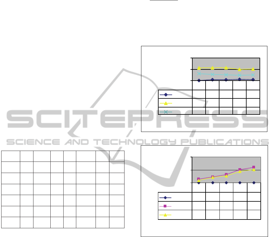
Figure 3 shows the construction times of these

algorithms. Naturally, Gp runs fastest since it is the

simplest and only the first portion of other

algorithms. We can see a significant reduction of

construction time by ROBE due to reduced number

of nodes and thus amount of pairwise distances

necessary to write on disk. The number of landmarks

indicated in the x-axis is the number of

representative nodes or popular nodes as a control

parameter. More structural data is shown in Table I,

where the column heads are number of marks,

number of representative nodes (rn), candidate

bridges (cand), chosen bridge nodes (bn), extension

nodes (en), number of components in G

, number of

super members (sm) and hub nodes (hub). In a dense

graph such as the one from SNAP, there are quite a

few super members in cliques. The compression rate

is roughly half.

Figure 4 shows the error rate, defined as

)(













where k is the total number of randomly generated

queries,





, and



are the estimated and true

distance of i

query.

0,5

#landmarks

Errorrate

Robe

0,009 0,043 0,042 0,06 0,048

Central

0,564 0,568 0,569 0,5 0,513

Constrai

0,31 0,274 0,257 0,24 0,251

10 20 30 40 50

Figure 3: Construction times of different schemes.

1000

2000

#landmarks

ConstructionTime(sec)

Robe

0,49 1,56 1,562 1,81 3,18

Central

279,5 464,4 632,4 1002 1199

Constrai

167,2 423,5 527,2 875 1001

10 20 30 40 50

Figure 4: Error rates of different schemes.

This measure reflects a relative, average error. The

error rate of Gp is the lowest (i.e. best) whenever the

distances can be estimated. However, if the distance

cannot be measured, a miss occurs. The query miss

happens either they are too far away or the chosen

subgraph is disconnected though they are originally

connected in the input graph.

From Figure 5, we find that more than half of the

queries are missed in Gp, which is normally

unacceptable. When we add bridges nodes and

extension nodes, the miss rate is greatly reduced. If

we do not limit the number of representative nodes,

the miss rate is zero. Most importantly, both

algorithms ROBE and G

have the same low error

rate and zero miss rate but ROBE is much faster due

to effective compression.

ICEIS2015-17thInternationalConferenceonEnterpriseInformationSystems

104

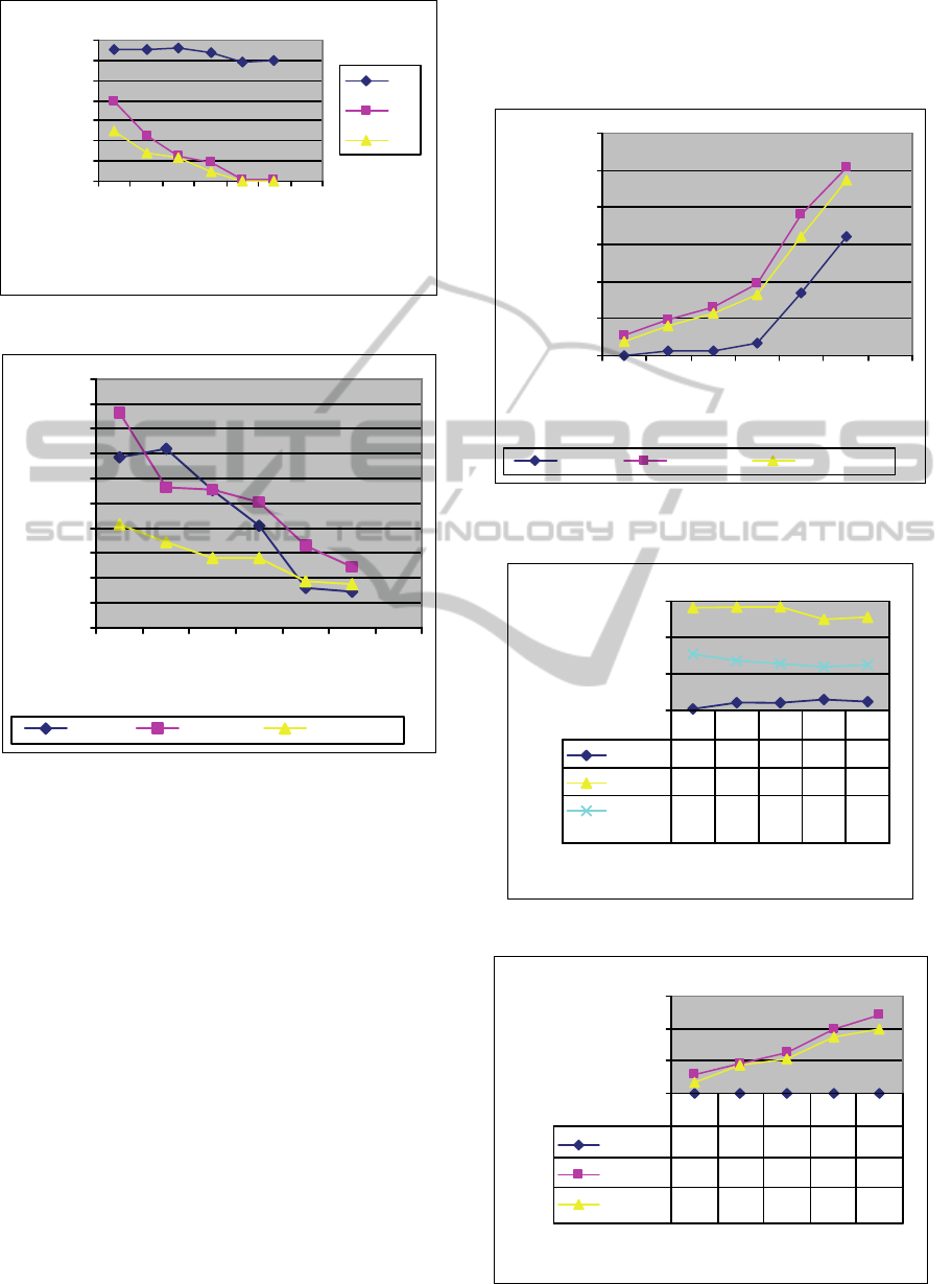
0.1

0.2

0.3

0.4

0.5

0.6

0.7

150

400

#landmarks

Miss Rate

Figure 5: Miss rate of different schemes.

0.02

0.04

0.06

0.08

0.1

0.12

0.14

0.16

0.18

0.2

50 100 150 200 400 600

#landmarks

Error Rate

Robe Central Constraint

Figure 6: Error rates of ROBE, Central, and Constraint

schemes.

In our next group of experiments we compare the

performance and error rate with two other recent

algorithms called Central and Constraint described

in (Potamias, Bonchi et al. 2009). In Central, from a

random set of seeds, a set of landmarks are chosen

so that their average distances to all other nodes in

the input graph are smallest. In Constraint, a number

of landmarks with the largest degrees are chosen so

that they are not next to one another. The critical

difference between ROBE and the other two

algorithms is that ROBE estimates the distance using

a chosen (much smaller) subgraph of the given input

graph while Central and Constraint need to compute

the distances from their global landmarks to all the

nodes in the input graph. Distance from u to v is

estimated as min{ distance(u, l

)+distance(v, l

)}

where the minimum is for each of the global mark l

Figures 6 and 7 illustrate the error rates and

construction times for different numbers of

landmarks. We can clearly see that ROBE greatly

reduces the construction time (two orders faster)

while maintaining similar or better error rates than

Central and Constraint. Among the latter two, in

general Constraint is better than Central.

10000

20000

30000

40000

50000

60000

50 100 150 200 400 600

#landm arks

Construction Time (ms)

Ro b e Central Constraint

Figure 7: Construction times of ROBE, Central, and

Constraint schemes.

0.2

0.4

0.6

#landmarks

Errorrate

Robe

0.009 0.043 0.042 0.06 0.048

Central

0.564 0.568 0.569 0.5 0.513

Constrai

0.31 0.274 0.257 0.24 0.251

10 20 30 40 50

Figure 8: Error rates for large data set.

500

1000

1500

#landmarks

ConstructionTime(sec)

Robe

0.49 1.56 1.56 1.81 3.18

Central

280 464 632 1002 1199

Constrai

167 424 527 875 1001

10 20 30 40 50

Figure 9: Construction times for large data set.

ROBE-KnittingaTightHubforShortestPathDiscoveryinLargeSocialGraphs

105

Lastly, we conduct a similar comparison on a much

larger, more realistic data set data-UCI provided by

University of California, Irvine (Gjoka , Gjoka,

Kurant et al. 2011). The graph has 1,189,768 nodes,

29,760,300 edges, one component, with an average

degree of 50 and maximal degree of 4,411. The

results are shown in Figures 8 and 9. Similar

observations can be made. The advantages of ROBE

are even more evident

7 CONCLUSIONS

In this work we have proposed and investigated a

technique called ROBE, which is based a hub

containing representative nodes, bridge nodes, and

extension nodes. Graph compression techniques

including clique compression, chain collapsing, and

tentacle retracting are exploited in order to reduce

the size and overall computation for the hub.

If all eligible representative nodes are chosen,

our scheme has a zero miss rate. Otherwise, its miss

rate is still very low. It also enjoys a low error rate,

in addition to its short construction time and low

cost for shortest-path queries. We have detailed our

design and performed extensive evaluations of

ROBE with related schemes and experimented on

two real data sets. The results suggest that ROBE

can serve as a good candidate for shortest-path

computation in large social networks.

REFERENCES

Agrawal, R. and R. Srikant (1994). Fast Algorithms for

Mining Association Rules in Large Databases.

VLDB'94, Proceedings of 20th International

Conference on Very Large Data Bases, September 12-

15, 1994, Santiago de Chile. J. B. Bocca, M. Jarke and

C. Zaniolo, Morgan Kaufmann: 487-499.

Akiba, T., Y. Iwata and Y. Yoshida (2013). Fast Exact

Shortest-Path Distance Queries on Large Networks by

Pruned Landmark Labeling. SIGMOD. New York.

Apostolico, A. and G. Drovandi ( 2009). "Graph

Compression by BFS." Algorithms 2: 1031-1044.

Backstrom, L., P. Boldi, M. Rosa, J. Ugander and S.

Vigna (2012). Four degrees of separation. WebSci.

Evanston, IL, USA: 33-42.

Baswana, S. and S. Sen (2006). "Approximate Distance

Oracles for Unweighted Graphs in Expected O(n^2)

Time." ACM Transactions on Algorihms 2(4): 557-

577.

Bellman, R. (1958). "On a routing problem." Quarterly of

Applied Mathematics (16): 87–90.

Chen, Z., Y. Chen, C. Ding, B. Deng and X. Li (2011).

Pomelo: accurate and decentralized shortest-path

distance estimation in social graphs. ACM SIGCOMM

Conference. Toronto, ON, Canada: 406-407.

Cohen, E., E. Halperin, H. Kaplan and U. Zwick (2003).

"Reachability and distance queries via 2-hop labels."

SIAM J. Comput. 32(5): 1338–1355.

Dijkstra, E. W. (1959). "A note on two problems in

connexion with graphs." Numerische Mathematik 1(1):

269–271.

Fan, W., J. Li, X. Wang and Y. Wu (2012). Query

preserving graph compression. SIGMOD. Scottsdale,

Arizona, USA: 157-168.

Feder, T. and R. Motwani (1995). "Clique partitions,

graph compression and speeding-up algorithms."

Journal of Computer And System Sciences 51: 261-

272.

Gao, J., R. Jin, J. Zhou, J. X. Yu, X. Jiang and T. Wang

(2011). Relational approach for shortest path

discovery over large graphs. Proc. VLDB Endow.

Gjoka, M. from http://odysseas.calit2.uci.edu/doku.php/

public:online_social_networks.

Gjoka, M., M. Kurant, C. T. Butts and A. Markopoulou

(2011). "Practical Recommendations on Crawling

Online Social Networks." IEEE J. Sel. Areas Commun.

on Measurement of Internet Topologies 29(9): 1872-

1892.

Gubichev, A., S. Bedathur, S. Seufert and G. Weikum

(2010). Fast and Accurate Estimation of Shortest

Paths in Large Graphs. CIKM, Toronta, Ontario,

Canada.

Jin, R., N. Ruan, Y. Xiang and V. E. Lee (2012). A

highway-centric labeling approach for answering

distance queries on large sparse graphs. SIGMOD:

445-456.

Jin, R., Y. Xiang, N. Ruan and D. Fuhry. . In ’09 (2009).

3-hop: a high-compression indexing scheme for

reachability query. SIGMOD.

Karande, C., K. Chellapilla and R. Andersen (2009).

Speeding up algorithms on compressed web graphs.

Proceedings of the Second ACM International

Conference on Web Search and Data Mining,

Barcelona, Spain.

Potamias, M., F. Bonchi, C. Castillo and A. Gionis (2009).

Fast shortest path distance estimation in large

networks. Proceedings of the 18th ACM conference on

Information and knowledge management. Hong Kong,

China: 867-876.

Qiao, M., H. Cheng, L. Chang and J. X. Yu (2012).

Approximate Shortest Distance Computing: A Query-

Dependent Local Landmark Scheme. ICDE,

Washington, DC, USA (Arlington, Virginia), 1-5

April, 2012.

Ruan, N., R. Jin and Y. Huang (2011). Distance

Preserving Graph Simplification.. ICDM. Vancouver,

Canada 1200-1205.

Sarma, A. D., S. Gollapudi, M. Najork and R. Panigrahy

(2010). A Sketch-Based Distance Oracle for Web-

Scale Graphs. WSDM, New York, USA.

SNAP. (2009). from http://snap.stanford.edu/data/.

Thorup, M. and U. Zwick (2005). "Approximate Distance

Oracles." Journal of the ACM 52(1): 1-24.

ICEIS2015-17thInternationalConferenceonEnterpriseInformationSystems

106

Wei, F. (2011). "TEDI: Efficient Shortest Path Query

Answering on Graphs." Graph Data Management:

Techniques and Applications: 214-238.

Zhao, X., A. Sala, C. Wilson, H. Zheng and B. Zhao

(2010). Orion: shortest path estimation for large social

graphs. Proceedings of the 3rd conference on Online

social networks. Boston, MA: 9-9.

ROBE-KnittingaTightHubforShortestPathDiscoveryinLargeSocialGraphs

107