
Open Framework for Combined Pedestrian Detection
Floris De Smedt and Toon Goedem´e
EAVISE, KU Leuven, Sint-Katelijne-Waver, Belgium
Keywords:
Pedestrian Detection, Real-time, Framework.
Abstract:
Pedestrian detection is a topic in computer vision of great interest for many applications. Due to that, a large
amount of pedestrian detection techniques are presented in current literature, each one improving previous
techniques. The improvement in accuracy in recent pedestrian detection, is commonly in combination with
a higher computational requirement. Although, recently a technique was proposed to combine multiple de-
tection algorithms to improve accuracy instead. Since the evaluation speed of this combination is dependent
on the detection algorithm it uses, we provide an open framework that includes multiple pedestrian detection
algorithms, and the technique to combine them. We show that our open implementation is superior on speed,
accuracy and peak memory-use when compared to other publicly available implementations.
1 INTRODUCTION
Pedestrian detection is a subject of great interest in
recent literature. Over the years a lot of work has
been performed on both speed (Doll´ar et al., 2010;
Benenson et al., 2012; Doll´ar et al., 2014; De Smedt
et al., 2013), and accuracy (Benenson et al., 2013;
Park et al., 2010). Although most of these techniques
are based on similar detection techniques, the con-
tribution they propose are applied on a single pedes-
trian detector. These improvements come mostly with
an extra computational requirement which is not al-
ways available. Recently, (De Smedt et al., 2014)
proposed an alternative technique to improve accu-
racy by combining the detection results of multiple
detectors. Their work uses only the detection results
neglecting the evaluation speed of the detection algo-
rithms themself. In this paper we propose an open
framework that provides the whole pipeline, from the
image to running multiple object detection algorithms
and finally the combination of their results. By re-
ducing the computational requirement of the pedes-
trian detection algorithms, the combination they are
part of will also come at a limited computational cost.
Therefor we compare our algorithms with other pub-
licly available implementations on speed, accuracy
and peak memory-use, and show that our implemen-
tations turn out to be superior based on these criteria.
The paper is structured as follows: In section 2 we
give an overview of existing literature. In section 3
we discuss the implementation of the pedestrian de-
tection algorithms we implemented. In section 4 we
give a detailed insight on how to combine the detec-
tion results. And finally we conclude in section 5.
2 RELATED WORK
Due to the wide applicability of pedestrian detec-
tion in a variety of applications (traffic, surveillance,
robotics and safety), their has been a lot of research
on this topic. In 2005 (Dalal and Triggs, 2005) pro-
posed a technique of using gradient information for
this task. They use a grid of HOG-features trained
with a linear Support Vector Machine, which imposed
impressive detection results on the INRIA pedes-
trian dataset. Datasets from more realistic conditions
(such as the Caltech pedestrian dataset (Doll´ar et al.,
2012b)) showed room for improvement on both accu-
racy and speed.
We can distinguish two fundamental techniques to
improve the accuracy of this detector. The model can
be extended, so instead of using a rigid model that
searches only for the object as a whole, the model also
includes parts (e.g. the limbs of a person). By allow-
ing a limited position deviation of the parts relatively
to the root model, a certain pose variation is allowed
(Felzenszwalb et al., 2008). On the other hand, one
can enrich the features used for pedestrian detection
by using color information next to gradient informa-
tion. This has been done in Integral Channel Features
proposed by (Doll´ar et al., 2009).
551
De Smedt F. and Goedemé T..
Open Framework for Combined Pedestrian Detection.
DOI: 10.5220/0005359205510558
In Proceedings of the 10th International Conference on Computer Vision Theory and Applications (VISAPP-2015), pages 551-558
ISBN: 978-989-758-090-1
Copyright
c
2015 SCITEPRESS (Science and Technology Publications, Lda.)

(Doll´ar et al., 2012b) and (Benenson et al., 2014)
give an overview of over 40 different pedestrian de-
tection algorithms in literature, discussing their eval-
uation methodology and accuracy. Here we see that
most of these techniques are based on the two al-
gorithms we discussed before. One of the most ac-
curacte algorithms is described in (Benenson et al.,
2013), where each step of the training process of In-
tegral Channel Features is evaluated and optimised.
This detector forms the base of (Mathias et al., 2013)
which copes with occlusion.
To allow the use of pedestrian detection in ap-
plications, both speed and accuracy need to be very
high. The speed can be improved by (a combina-
tion of) three approaches. One can use more capa-
ble hardware such as GPU or multi-core CPU to ex-
ploit parallellisation, as has been done by (Benen-
son et al., 2012; De Smedt et al., 2012; De Smedt
et al., 2013). Constraining the appearances to a limit-
ted amount of sizes and positions by using ground
plane assumption and/or tracking reduces the search-
ing space (De Smedt et al., 2013; Benenson et al.,
2012), and thereby the calculation time needed. A last
option is to optimise the algorithms themself. Some
examples are approximating features from calculated
ones (Doll´ar et al., 2014; Doll´ar et al., 2010), learn
a model for each scale (Benenson et al., 2012), us-
ing a cascaded evaluation(Felzenszwalb et al., 2010a;
Bourdev and Brandt, 2005) and using Crosstalk Cas-
cade where the detection results at nearby locations
is exploited (and so reducing the amount of locations
evaluated) (Doll´ar et al., 2012a).
To allow the use of these algorithms, some of the
implementations are made publicly available. The
implementations of (Benenson et al., 2012; Benen-
son et al., 2013; Benenson et al., 2014) are com-
bined in a single framework
1
. This framework is
mostly directed to using a (modern) GPU for fast
processing, while using very accurate detection ap-
proaches. (Dubout and Fleuret, 2012) made the code
available
2
for an optimised version of the Deformable
Part Model detector, as described in (Felzenszwalb
et al., 2008). In contrast to (Felzenszwalb et al.,
2010a), where a cascade-approach is used for speed
improvement, they make use of multi-threading and
apply convolution in the Fourier-domain as a dot-
product. Altough, this implementation comes at the
cost of high memory-use, as we will point out in sec-
tion 3. The availability of GPU and high memory
restricts the applicability of these frameworks on for
example embedded systems. In this paper we pro-
pose a complementary framework focussing on cpu-
1
https://bitbucket.org/rodrigob/doppia
2
http://charles.dubout.ch/en/coding.html
implementations at limited memory-use.
Recently (De Smedt et al., 2014) proposed a tech-
nique to even further improve the accuracy. Instead of
tuning a single object detection algorithms, they com-
bine the strenghts of different algorithms by combin-
ing the detection results. They use the measurement
of confidence (how trustworthy is a detection of a cer-
tain detector) and complementarity (how different are
two detectors, so how likely is it they result in the
same detections) to combine the detecions scores in
a weighted sum. Since the score-range between de-
tectors can vary drastically, they use a normalisation
step based on the average and mean of the scores. In
this paper we apply this technique on our implemen-
tations as an alternative for a computational intensive
single tuned algorithm.
3 IMPLEMENTATION OF
OBJECT DETECTION
ALGORITHMS
Each choice that is made in the construction of an
object detection algorithm influences the final results
it will obtain. In (Benenson et al., 2013) for exam-
ple, is shown how optimising each step of the training
procedure of Integral Channel Detector (Doll´ar et al.,
2009) can lead to a drastic improvement in accuracy
(coined the Roerei-detector). The distinguishability
of features and structure of the model is bound to the
dimension reduction it imposes on the huge search-
ing space to find pedestrians. Next to that, is also
the computational complexity, and by consequence
the evaluation speed, of great importance when real-
time execution is required. As is shown in (De Smedt
et al., 2014), each detector has its own strenghts and
weaknesses due to the differences in design, and will
also lead to different detection results. They provide
a technique to combine the detection results of mul-
tiple pedestrian detectors to improve detection accu-
racy, in contrast to the traditional approach of improv-
ing a single detector with higher computational cost
as a consequence. The cost of combining multiple
detection algorithms depends on the algorithms them-
selves. In this section we describe the pedestrian de-
tection algorithms we implemented in our framework,
and compare them on speed, peak memory-use and
accuracy. Based on this comparison, we make pair-
wise combinations of pedestrian detection algorithms
in section 4.
VISAPP2015-InternationalConferenceonComputerVisionTheoryandApplications
552
3.1 Traditional Object Detection
Approach
The approach to distinguish the appearance of an ob-
ject from the background is a difficult task, mostly
solved in the same sequence of steps. The image is
rescaled multiple times, to obtain the detections at
multiple scales. Rescaling the model (or obtaining
a model for different scale appearances of the ob-
ject) is discussed in (Benenson et al., 2012), and is
far more complex than rescaling the image instead.
For each scale certain features are calculated to em-
phasise properties of the image capable to distinguish
the object from the background. The last step is to
express the similarity between the features and a pre-
trained model as a numeric value. All the detections
with a score above a chosen threshold will be seen
as containing the object, where the ones below the
threshold are treated as background information. A
high threshold will lead to only a few detections, but
also less false detections (a high precision), where a
low threshold ensures that more appearences of the
object will be found, but also more false detections
will be made (high recall). The accuracy of an object
detection algorithm for different thresholds can be ex-
pressed in a precision-recall curve. We use this kind
of curve extensively in this paper, an example can be
seen in figure 3.
3.2 Histogram of Oriented Gradients
The first algorithm we integrated in our framework
is Histogram of Oriented Gradients (HOG). This
technique, described in (Dalal and Triggs, 2005) for
pedestrian detection, makes use of contrast informa-
tion of the image to recognise the appearance of
pedestrians. The model used here, forms the root-
model for the Deformable Part Models-detector and
is shown in figure 2 at the left. The implementation
we use is part of OpenCV. For speed improvement,
they use a very similar approach as we do, by evaluat-
ing the layers of the scale-space-pyramid in parallel.
For integration in our framework, we convert the de-
tection results to our format. To allow a fair compar-
ison with the other algorithms, we use our own Non-
Maximum suppression implementation instead of the
one provided by OpenCV.
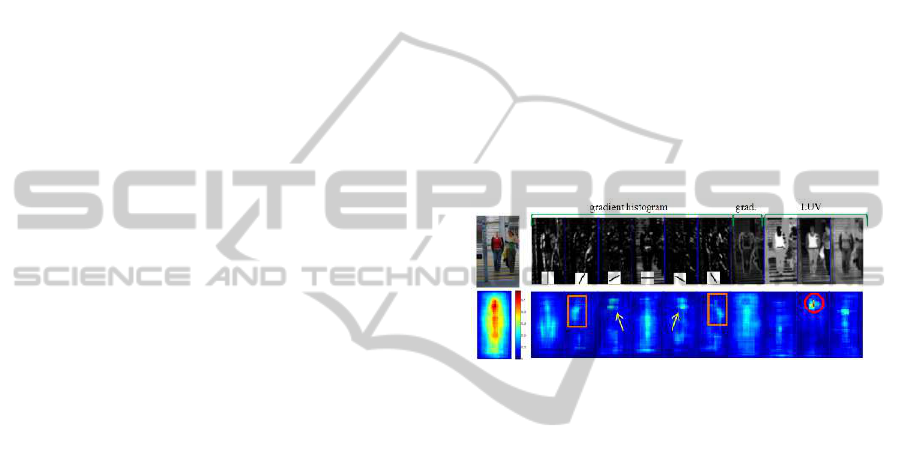
3.3 Integral Channel Features
As described in section 2, the Integral Channel Fea-
tures detector makes use of multiple features for ob-
ject detection. Each feature is presented as a chan-
nel. In the original implementation, 10 channels are
used (6 gradient orientation, 1 gradient magnitude
and 3 colour channels). These are shown in figure 1.
The model is constructed from a selection of rectan-
gles containing the sum of the intensity values from a
channel. The rectangles are selected from a huge pool
of random rectangles using Adaboost. To improve
the speed, we use softcascade (Bourdev and Brandt,
2005) so that after the evaluation of each feature, the
current score is required to reach a pre-determined
treshold to continue the evaluation at that location.
To find the annotation, it is required that the detec-
tion bounding box has an overlap of at least 50% with
the annotation. The selection of the threshold used for
softcascade determines the resulting balance between
accuracy and speed. A high threshold will lead to
more pruning, so higher speed, where a lower thresh-
old is more indulgent and will allow more detections
to reach the final stage at the cost of evaluation speed.
Figure 1: The channels used in the original implementation
of (Doll´ar et al., 2009).
To calculate the features, we use the code released
as part of the ACF-implementation of (Doll´ar et al.,
2014), which is heavily optimised for cpu (Doll´ar,
2013). To improve accuracy, the model used for eval-
uation is trained with an extra space around the anno-
tation. After detection, the bounding box is altered to
the original dimensions, which better fits the object.
The accuracy and evaluation speed of our implemen-
tation are discussed in subsection 3.5.
3.4 Deformable Part Models
The Deformable Part Model detector we use is based
on the vanilla implementation used by (De Smedt
et al., 2012) and (De Smedt et al., 2013). It is a
C++-port of the matlab implementation of DPMv4 re-
leased in (Felzenszwalb et al., 2010b). Deformable
Part Models can be seen as an extension of the HOG-
model used by (Dalal and Triggs, 2005) with part
models. The evaluation of the model can be divided
in the search for the root model, representing the ob-
ject as a whole, and the search for parts (e.g. the limbs
of a person). The location of the part models relative
to the position of the root model can deviate a litte,
to allow a certain pose variation in contrast to rigid-
model detectors. The model we use is trained on the
OpenFrameworkforCombinedPedestrianDetection
553
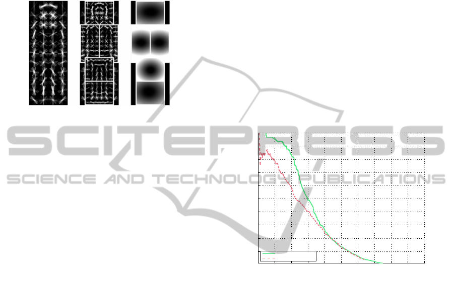
INRIA-dataset and is visualized in figure 2. Since the
part models are a more detailed element of the object,
they are searched for at twice theresolution as the root
model. This imposes the choice of 3 different imple-
mentation approaches to obtain features at twice the
size.
Figure 2: The model used by (Felzenszwalb et al., 2008;
Felzenszwalb et al., 2010a). The root-model at the left, the
part-models in the middle and the allowed deviation at the
right.
The most intuitive manner is to upscale the im-
age where the root model is searched on (coined DPM
Up). Altough the information contained in an image
can not be extended, the stability of the model can
benefit from this. Another option is to do the oppo-
site, and downscale the image used for the part filters
instead (coined DPM Down). Since downscaling is
faster than upscaling (both in memory as in compu-
tational complexity), this seems a good option. Al-
though it comes with a pitfall. The object can only be
found at twice the original size of the model. To ob-
tain the same scale range as the previous design, we
have to upscale the image to twice the resolution up
front, which takes away the advantage. The last op-
tion is to not rescale at all, but use half the amount of
pixels to calculate the histogram (coined DPM Half).
These three implementation methods are discussed in
subsection 3.5, and as can be seen, only the use of tak-
ing half the cell-size comes with a minimal accuracy
loss, while being a lot less computationally intensive.
We optimised our implementation by eliminating
redundant work, exploit locality in memory and avoid
global memory for thread-safe code. This allows us
to evaluate the layers of the scale-space-pyramid in
parallel.
3.5 Speed, Memory and Accuracy
In the previous subsections, we described three al-
gorithms seperately. The choice of which algorithm
to use independently, or as part of a combination, is
based on memory-use, evaluation time and the accu-
racy. To evaluate these criteria, we use the evalua-
tion framework of (Doll´ar et al., 2012b; Doll´ar, 2013)
at a Reasonable setting (50px and higher, with max
45% occlusion). The 120px height of the Deformable
Part Model-model imposes the requirement to per-
form an initial upscale of 2.4 times (we round to 2.5
times) to obtain detections at 50px. Therefor, we also
evaluate the speed and memory-use at different im-
age sizes. All experiments are performed on the same
platform. The amount of parallellisation influences
both the evaluation speed and memory-use, but the
accuracy remains constant.
The HOG-implementation of OpenCV (which we
use) has the model embedded in the code, in contrast
to our algorithms that uses a text-file. The accuracy
we obtain is visualised in figure 3. As we can observe,
the OpenCV-implementation improves its accuracy at
higher threshold compared to the original accuracy re-
sults.
0 0.1 0.2 0.3 0.4 0.5 0.6 0.7 0.8 0.9 1
0.1
0.2
0.3
0.4
0.5
0.6
0.7
0.8
0.9
1
Recall
Precision
Comparison of standard HOG with OpenCV implementation
70.62% HOG−OpenCV
58.38% HOG
Figure 3: Accuracy comparison between the original HOG
and the implementation of OpenCV we use.
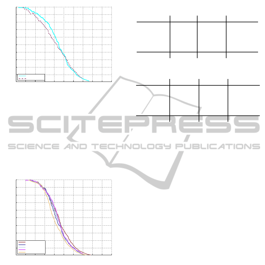
We trained an Integral Channel Features model
ourself, based on the INRIA pedestrian training set.
The complete images are used instead of the nor-
malised ones, and each annotation is rescaled to
41x100 pixels (size of our inner-model). The outer-
model (annotation + extra spacing) is chosen to be
64x128 pixels, as has been done in the ACF-training
code of (Doll´ar et al., 2014; Doll´ar, 2013). We used
a 2048 stage model, where each stage is a level-two
decision tree as weak classifier. To obtain a complete
PR-curve, we used a permissive threshold for softcas-
cade. In figure 4 we compare the accuracy results we
obtain with the ones in the framework, as obtained
by (Doll´ar et al., 2009). We can observe that our im-
plementation performs slightly better compared to the
original Matlab implementation.
The model used for our Deformable Part Model
detector is also trained on INRIA, and comes with the
original Matlab release (Felzenszwalb et al., 2010b).
We used a matlab-script to convert the .mat-file to
a textfile which can be used by our implementation.
VISAPP2015-InternationalConferenceonComputerVisionTheoryandApplications
554
0 0.1 0.2 0.3 0.4 0.5 0.6 0.7 0.8 0.9 1
0.1
0.2
0.3
0.4
0.5
0.6
0.7
0.8
0.9
1
Recall
Precision
Comparison of standard Integral Channel Features with our implementation.
76.43% ICF−Ours
75.78% ChnFtrs
Figure 4: Accuracy comparison between our implemen-
tation of Integral Channel Features and the results from
(Doll´ar et al., 2009).
This is a model of 40x120 pixels. As described in
subsection 3.4, there are 3 methods to obtain the fea-
tures for the evaluation of the root-model and the
part-models. In figure 5 we compare these 3 options
with the original Matlab-implementation (Latv4-cc)
and the implementation of (Dubout and Fleuret, 2012)
(FFLD). As we can see, the accuracy results we ob-
tain are all very similar.
0 0.1 0.2 0.3 0.4 0.5 0.6 0.7 0.8 0.9 1
0.1
0.2
0.3
0.4
0.5
0.6
0.7
0.8
0.9
1
Recall
Precision
Comparison of Deformable Part Models implementations
78.23% FFLD
77.49% DPM−Half
77.38% DPM−Up
77.36% DPM−Down
76.53% Latv4−cc
Figure 5: Comparison of the accuracy results of Deformable
Part Models.
In table 1 and table 2 we compare the evaluation
speed and memory-use respectively, of each imple-
mentation of our framework. The improvement in ac-
curacy for both Deformable Part Models and Integral
Channel Features over Histogram of Oriented Gradi-
ents comes at the cost of speed loss and higher peak
memory-use. When we compare our implementations
of Deformable Part Models, we can point out that we
only need a fraction of the memory needed by FFLD,
while using half the cell-size is more than twice as
fast on VGA-resolution.
Based on the criteria we just evaluated, we can
Table 1: Comparison of evaluation speed of the algorithms
we provide.
640x480 1280x960 1600x1200
HOG 15.1 fps 4.1 fps 2.66 fps
ICF
10.71 fps 2.12 fps 1.37 fps
DPM Half
8.63 fps 1.30 fps 0.82 fps
DPM Up
5.58 fps 0.82 fps 0.45 fps
DPM Down
2.98 fps 0.74 fps 0.48 fps
FFLD 3.828 fps 0.96 fps 0.67 fps
Table 2: Comparison of memory-use when running the
pedestrian detection algorithms.
640x480 1280x960 1600x1200
HOG 42.9MB 141.5 MB 243.4 MB
ICF
163.1 MB 446.4 MB 659.4 MB
DPM Half
82.72 MB 240.3 MB 429.2 MB
DPM Up
102 MB 253 MB 442 MB
DPM Down
120 MB 332.6 MB 537.2 MB
FFLD 790 MB 3.0 GB 4.7 GB
select the best pair of detectors to combine. For accu-
racy, it will be better to combine our Integral Channel
Feature-detector with our Deformable Part Models-
detector, while for speed it may be a better choice to
combine Histogram of Oriented Gradients with Inte-
gral Channel Features. In section 4 we discuss how
to combine detectors, and evaluate the combinations
on the same criteria (evaluation speed, peak memory-
use and accuracy) for the pairwise combinations of
our implementations.
4 COMBINATION
In this section, we will discuss how to combine the
detectors we described in section 3. The steps to
obtain a combined detection result are visualized in
figure 6. The first steps are performed as described
in section 3, where a scale-space-pyramid is created
from the source image. Each layer of the scale-space
pyramid is then processed by a pedestrian detection
algorithm. The next step is to normalise the detec-
tion scores. This is required, since each detector has a
different score-range. The normalisation of detection
scores is described in subsection 4.1. After normali-
sation, we have multiple options. We can just throw
the detections (before NMS) in one big pool and treat
them as coming from a single detector. This is de-
scribed in subsection 4.2. A more accurate alternative
is performing a smart combination from the detection
results after NMS, which is described in subsection
4.3.
OpenFrameworkforCombinedPedestrianDetection
555
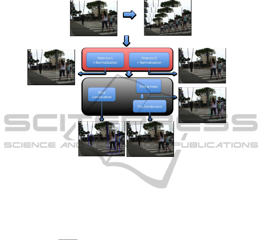
Figure 6: Overview of combination approach.
4.1 Normalisation
The normalisation of detection scores is necessary,
since the range of detection scores can differ drasti-
cally between different detection algorithms. Here we
use the standard score approach as has been used by
(De Smedt et al., 2014). The equation looks as fol-
lows:
S
norm
=
(S− µ
s
)
σ
s
This results in all detection scores being positions
around the zero-value. For this approach a working
point has to be defined and all detections with detec-
tion score above the working point are taken into ac-
count to calculate the mean and standard deviation.
Next to the score, we also have to equalise the as-
pect ratio of the bounding boxes between the detec-
tors. The aspect ratio between ICF and DPM (Inte-
gral Channel Features and Deformable Part Models)
differ slightly. We empirically found out that altering
the bounding boxes by keeping the height constant,
turns out to aquire the best accuracy results.
4.2 Pool Combination
With the normalised scores, we can treat the resulting
detections of all detectors equally. This means that
we can just put the detections together into the same
pool and perform Non-Maximum suppression over
all detections found with multiple detectors. As we
will show in section 4.4, the accuracy results depend
on the accuracy of the algorithms to combine. Due
to normalisation, the detectors are treated equally, so
the accuracy difference is lost. The combination ap-
proach described in section 4.3 takes this difference
into account in the form of the confidence value.
4.3 The Combinator
Recently (De Smedt et al., 2014) proposed a tech-
nique to combine the results of different object de-
tection algorithm, which they apply for the detec-
tion of pedestrian detectors. The combined score
they obtained is formed by using a weighted sum
of normalised detection scores, where each score is
weighted by using two coeficients, the confidence and
the complementarity. The confidence is a measure-
ment to express how well a certain detector works on
itself, while the complementarity measures the differ-
ences between detection results. If detectors are based
on completely different feature pools, they most prob-
ably will result in different detections, meaning that a
combined detection has a higher chance of being cor-
rect, compared to very similar detectors leading to the
same detection. They use the following equation to
VISAPP2015-InternationalConferenceonComputerVisionTheoryandApplications
556
obtain the final detection score:
S
final
=
n
∑
i=1
c
conf(i)
c
compl(i)
(S
i
+ Q)
The Q added to the normalised score is required
when the Standard score approach is used for nor-
malisation, to avoid the presence of negative nor-
malised scores, which would lead to a decrease in the
weighted sum formula.
The same working point is used to aquire the mean
and standard deviation for normalisation (as described
in subsection 4.1) as to obtain the confidence and
complementarity coeficients. The confidence is de-
fined as the area between the origin and the working
point. Here, we simplify the weighted sum formula
by eliminating the use of a complementarity value,
since it has no additional information when used for a
pairwise combination.
4.4 Evaluation of Speed and Accuracy
Finally, we compare the implementations we have
proposed as part of our framework. The accuracy
of the object detection algorithms, and the models
we use, is already discussed in subsection 3.5, but
are shown again in comparison with the combina-
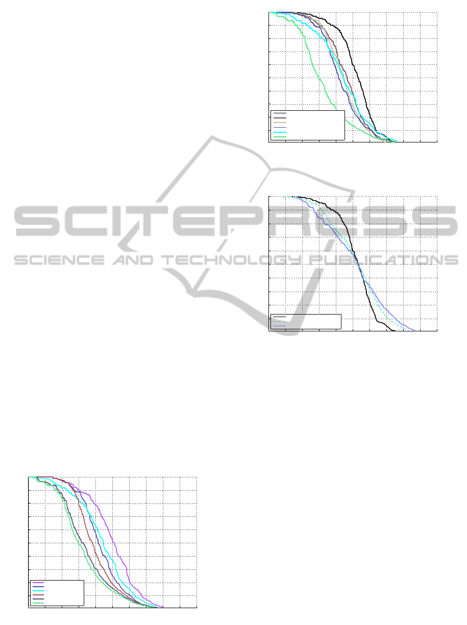
tion techniques we described earlier. In figure 7 we
compare the use of pool-combination as described in
subsection 4.2. As we can observe, the combination
of Histogram of Oriented Gradients with either De-
formable Part Models or Integral Channel Features
does not improve accuracy. This is due to the fact that
the accuracy-difference is ignored. When we com-
bine Integral Channel Features and Deformable Part
Models on the other hand, which have more or less an
equal accuracy, we obtain a big improvement in accu-
racy.
In figure 8, we compare the accuracy results we
0 0.1 0.2 0.3 0.4 0.5 0.6 0.7 0.8 0.9 1
0.1
0.2
0.3
0.4
0.5
0.6
0.7
0.8
0.9
1
Recall
Precision
Comparison of our implementations of Pool Combination
80.13% Pool−ICF+DPM
77.49% DPM−Half
76.43% ICF−Ours
76.04% Pool−HOG+DPM
71.71% Pool−HOG+ICF
70.62% HOG−OpenCV
Figure 7: Comparison of the accuracy of the implementa-
tions we propose.
0 0.1 0.2 0.3 0.4 0.5 0.6 0.7 0.8 0.9 1
0.1
0.2
0.3
0.4
0.5
0.6
0.7
0.8
0.9
1
Recall
Precision
Comparison of our implementations of The Combinator
81.48% Combinator−ICF+DPM
78.20% Combinator−HOG+ICF
78.00% Combinator−HOG+DPM
77.49% DPM−Half
76.43% ICF−Ours
70.62% HOG−OpenCV
Figure 8: Comparison of the accuracy of the implementa-
tions we propose.
0 0.1 0.2 0.3 0.4 0.5 0.6 0.7 0.8 0.9 1
0.1
0.2
0.3
0.4
0.5
0.6
0.7
0.8
0.9
1
Recall
Precision
81.48% TheCombinatorICFDPM
81.18% Roerei
80.23% MultiResC
Figure 9: Comparison of the our most accurace combina-
tion with the state-of-the-art.
obtain by using the smarter combination approach de-
scribed in subsection 4.3. Here we can point out that
the accuracy benefits from combining. The additional
value of Histogram of Oriented Gradients is not that
big though.
Table 3 and table 4 show the evaluation speed and
peak memory-userespectively of our combination ap-
proaches. As we can point out, the evalutation speed
and peak-memory of a combination is dependend on
the slowest algorithm in the combination. When for
example Integral Channel features is combined with
Deformable Part Models, part of the CPU-cores are
assigned to the Deformable Part Models algorithm.
Since Deformable Part Models does not need as much
memory, the peak memory-use is less then the sum of
Integral Channel Features and Deformable Part Mod-
els seperately.
When we compare the combination of De-
formable Part Models and Integral Channel Features
with the state-of-art detectors (figure 9), it can be seen
that a combination reaches impressive accury results.
Altough the PR-curve crosses the ones of Roerei (Be-
OpenFrameworkforCombinedPedestrianDetection
557

nenson et al., 2013) and MultiRes (Park et al., 2010),
it is only at the point where only half the detec-
tions are correct (precision of 0.5). For most appli-
cations the required precision is significantly higher.
For MultiRes, no evaluation speed is mentioned in
(Park et al., 2010), and (Benenson et al., 2013) (the
Roerei-detector) claims an evaluation speed of 5Hz-
20Hz while using GPU-hardware.
Table 3: Comparison of evaluation speed of the combined
algorithms.
640x480 1280x960 1600x1200
HOG 15.1 fps 4.1 fps 2.66 fps
ICF 10.71 fps 2.12 fps 1.37 fps
DPM Half
8.63 fps 1.30 fps 0.82 fps
Pool HOG+DPM 6.8 fps 0.57 fps 0.31 fps
Pool HOG+ICF 7.65 fps 1.60 fps 1.03 fps
Pool ICF+DPM 7 fps 0.54 fps 0.29 fps
Combinator HOG+DPM 6.8 fps 0.57 fps 0.31 fps
Combinator HOG+ICF 7.57 fps 1.57 fps 1.03 fps
Combinator ICF+DPM 6.78 fps 0.53 fps 0.29 fps
Table 4: Comparison of memory-use when running the
pedestrian detection algorithms.
640x480 1280x960 1600x1200
HOG 42.9MB 141.5 MB 243.4 MB
ICF 163.1 MB 446.4 MB 659.4 MB
DPM Half 82.72 MB 240.3 MB 429.2 MB
Pool HOG+DPM 80.2 MB 261 MB 424 MB
Pool HOG+ICF
162 MB 428 MB 657 MB
Pool ICF+DPM 105 MB 318 MB 505 MB
Combinator HOG+DPM 82.2 MB 264 MB 424 MB
Combinator HOG+ICF
174 MB 420 MB 694 MB
Combinator ICF+DPM 124 MB 336 MB 482 MB
5 CONCLUSION
In this paper we present for the first time a full-
pipeline implementation of detection combination as
an open framework. In contrast to the traditional ap-
proach of improving detection accuracy by optimis-
ing a single detector, we use a technique of com-
bining multiple pedestrian detectors instead, a tech-
nique proposed in (De Smedt et al., 2014). Herefor
we use the Histogram of Oriented Gradients imple-
mentation of OpenCV with our own implementation
of Integral Channel Features and of Deformable Part
Models. Based on the criteria of evaluation speed,
peak memory-use and accuracy, we obtained supe-
rior results to publicly available (CPU) implemen-
tations. The accuracy obtained by combining De-
formable Part Models with Integral Channel Features
is impressive compared to state-of-the-art detectors
which are far more computation intensive.
Code for this framework is available at http://
eavise.be/AbnormalBehaviour, and can be used for
research purposes.
REFERENCES
Benenson, R., Mathias, M., Timofte, R., and Van Gool, L.
(2012). Pedestrian detection at 100 frames per second.
In CVPR. IEEE.
Benenson, R., Mathias, M., Tuytelaars, T., and Van Gool, L.
(2013). Seeking the strongest rigid detector. In CVPR.
IEEE.
Benenson, R., Omran, M., Hosang, J., and Schiele, B.
(2014). Ten years of pedestrian detection, what have
we learned?
Bourdev, L. and Brandt, J. (2005). Robust object detection
via soft cascade. In CVPR, volume 2. IEEE.
Dalal, N. and Triggs, B. (2005). Histograms of oriented
gradients for human detection. In CVPR, volume 1.
IEEE.
De Smedt, F., Struyf, L., Beckers, S., Vennekens, J.,
De Samblanx, G., and Goedem´e, T. (2012). Is the
game worth the candle? evaluation of opencl for ob-
ject detection algorithm optimization. PECCS.
De Smedt, F., Van Beeck, K., Tuytelaars, T., and Goedem´e,
T. (2013). Pedestrian detection at warp speed: Ex-
ceeding 500 detections per second. In CVPRW. IEEE.
De Smedt, F., Van Beeck, K., Tuytelaars, T., and Goedem´e,
T. (2014). The combinator: optimal combination of
multiple pedestrian detectors. In ICPR.
Doll´ar, P. (2013). Piotrs image and video matlab toolbox
(pmt). Software available at: http://vision. ucsd. edu/˜
pdollar/toolbox/doc/index. html.
Doll´ar, P., Appel, R., Belongie, S., and Perona, P. (2014).
Fast feature pyramids for object detection. PAMI,
36(8).
Doll´ar, P., Appel, R., and Kienzle, W. (2012a). Crosstalk
cascades for frame-rate pedestrian detection. In
ECCV.
Doll´ar, P., Belongie, S., and Perona, P. (2010). The fastest
pedestrian detector in the west. In BMVC.
Doll´ar, P., Tu, Z., Perona, P., and Belongie, S. (2009). Inte-
gral channel features. In BMVC, volume 2.
Doll´ar, P., Wojek, C., Schiele, B., and Perona, P. (2012b).
Pedestrian detection: An evaluation of the state of the
art. PAMI, 34.
Dubout, C. and Fleuret, F. (2012). Exact acceleration of
linear object detectors. In ECCV. Springer.
Felzenszwalb, P., McAllester, D., and Ramanan, D. (2008).
A discriminatively trained, multiscale, deformable
part model. In CVPR. IEEE.
Felzenszwalb, P. F., Girshick, R. B., and McAllester, D.
(2010a). Cascade object detection with deformable
part models. In CVPR. IEEE.
Felzenszwalb, P. F., Girshick, R. B., and
McAllester, D. (2010b). Discriminatively
trained deformable part models, release 4.
http://people.cs.uchicago.edu/ pff/latent-release4/.
Mathias, M., Benenson, R., Timofte, R., and Gool, L. V.
(2013). Handling occlusions with franken-classifiers.
In ICCV. IEEE.
Park, D., Ramanan, D., and Fowlkes, C. (2010). Multireso-
lution models for object detection. In ECCV. Springer.
VISAPP2015-InternationalConferenceonComputerVisionTheoryandApplications
558
