Graph-based ETL Processes for Warehousing Statistical Open Data
Alain Berro, Imen Megdiche and Olivier Teste
IRIT UMR 5505, University of Toulouse, CNRS, INPT,
UPS, UT1, UT2J, 31062 Toulouse Cedex 9, France
Keywords:
Statistical Open Data, RDF Graphs, Tables Extraction, Holistic Integration, Multidimensional Schema.
Abstract:
Warehousing is a promising mean to cross and analyse Statistical Open Data (SOD). But extracting structures,
integrating and defining multidimensional schema from several scattered and heterogeneous tables in the SOD
are major problems challenging the traditional ETL (Extract-Transform-Load) processes. In this paper, we
present a three step ETL processes which rely on RDF graphs to meet all these problems. In the first step,
we automatically extract tables structures and values using a table anatomy ontology. This phase converts
structurally heterogeneous tables into a unified RDF graph representation. The second step performs a holistic
integration of several semantically heterogeneous RDF graphs. The optimal integration is performed through
an Integer Linear Program (ILP). In the third step, system interacts with users to incrementally transform the
integrated RDF graph into a multidimensional schema.
1 INTRODUCTION
Crossing and analysing Statistical Open Data (SOD)
in a data warehouse is a promising way to derive
several insights and reuse these miner sources of
information. Except that Open Data’ characteris-
tics make them unaffordable with traditional ETL
(Extract-Transform-Load) processes. Indeed, an im-
portant part
1
of governmental SOD holds into spread-
sheets disposing structurally and semantically hetero-
geneous tables. Moreover these sources are scat-
tered across multiple providers and even in the same
provider which hampers their integration.
To cope with these problems, we propose RDF-
based ETL processes composed of three steps which
adapt the extract, transform and load traditional ETL
steps. The first step gives a solution to the automatic
data table extraction and annotation problem. The
second one gives a solution to the automatic holistic
data integration problem. The third step focuses on an
incremental multidimensional schema definition from
the integrated RDF graphs. In this latter, we aim to
maintain the re-usability of processed SOD.
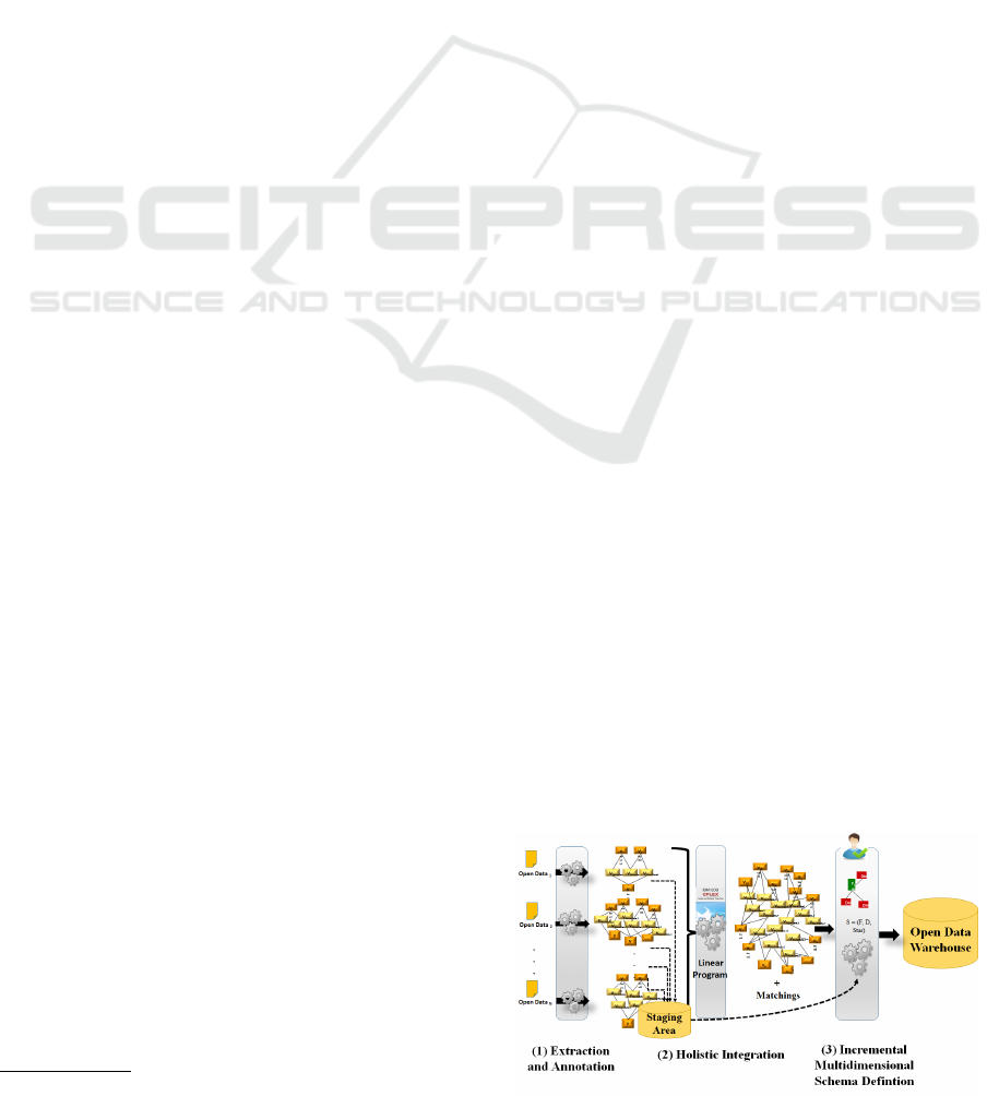
RDF Graph-based ETL Processes. Our ETL pro-
cesses are based on manipulating RDF graphs. They
are depicted in Fig.1 as follows:
1
http://fr.slideshare.net/cvincey/opendata-benchmark-
fr-vs-uk-vs-us
• Step 1: ”Extraction and Annotation”, it takes as
input flat SOD spreadsheets and provides as out-
put unified RDF instance-schema graphs. The
main challenge is to automatically identify and re-
structure data from spreadsheets tables in order to
be able to reuse them. We propose a workflow to
automatically perform the ETL extraction phase.
Each activity in the workflow extracts and anno-
tates table components guided by a table anatomy
ontology then constructs iteratively the vertices
and edges of the output graph. Finally, users val-
idate automatic annotations and the output graphs
are stored in a staging area.
• Step 2: ”Holistic Integration”, it takes as input
structural parts of several SOD RDF graphs and
generates as output an integrated RDF graph and
the underlying matchings. The integrated graph is
Figure 1: Graph-Based ETL Processes.
271
Berro A., Megdiche I. and Teste O..
Graph-based ETL Processes for Warehousing Statistical Open Data.
DOI: 10.5220/0005363302710278
In Proceedings of the 17th International Conference on Enterprise Information Systems (ICEIS-2015), pages 271-278
ISBN: 978-989-758-096-3
Copyright
c
 2015 SCITEPRESS (Science and Technology Publications, Lda.)

composed of collapsed and simple vertices con-
nected by simple edges. Collapsed vertices ref-
erence groups of matched vertices. Not matched
ones remain simple vertices. We propose a lin-
ear program to perform an automatic and optimal
holistic integration. Users can validate and/or ad-
just the proposed solution. The linear program
maximizes semantic and syntactic similarity be-
tween the labels of the vertices of the input graphs.
It also resolves conflictual matching situations in-
volving different graphs’ structures by ensuring
strict hierarchies (Malinowski and Zim
´
anyi, 2006)
and preserving logical edges directions.
• Step 3: ”Incremental Multidimensional Schema
Definition”, it takes as input an integrated graph
and generates as output a multidimensional
schema. An interactive process is established be-
tween users’ actions and system. On the one hand,
users’ actions consist on incrementally identify-
ing multidimensional components such as dimen-
sions, parameters, hierarchies, fact and measures.
On the other hand, system interacts with users’ ac-
tions by transforming identified components into
a multidimensional schema.
Motivating Example. The case study deals with an
agricultural company in England aiming at launching
a new project on cereal production. The company is
interested on analysing cereal production activity in
the previous years in UK. With a simple search on
the UK governmental provider https://www.gov.uk/,
the company retrieves relevant informations for this
topic. For instance the link
2
provides several detailed
sources for cereal production by cereal type, by farm
size, by farm type, and soon. These sources suffer
from the different problems presented above. They
are: (i) scattered into different spreadsheets even in
the same link, (ii) structurally heterogeneous since the
spreadsheets can have one or several tables disposed
randomly, and (iii) semantically heterogeneous due to
the different analysis axis influencing the agricultural
statistics.
The following sections describe the three steps of
our approach respectively in sections 2, 3, 4.
2 EXTRACTION AND
ANNOTATION
In this section, we describe a workflow performing
2
https://www.gov.uk/government/statistical-data-
sets/structure-of-the-agricultural-industry-in-england-and-
the-uk-at-june
Figure 2: The Open Data Tables Annotating Concepts.
extraction, annotation and transformation of flat open
data tables into RDF instance-schema graphs.
2.1 The Tables Annotating Ontology
In order to annotate tables, we have extended the ba-
sic table anatomy described by (Wang, 1996). A ta-
ble contains a body (a set of numerical data) indexed
by structural data which are StubHead (row headers)
and/or BoxHead (column headers).
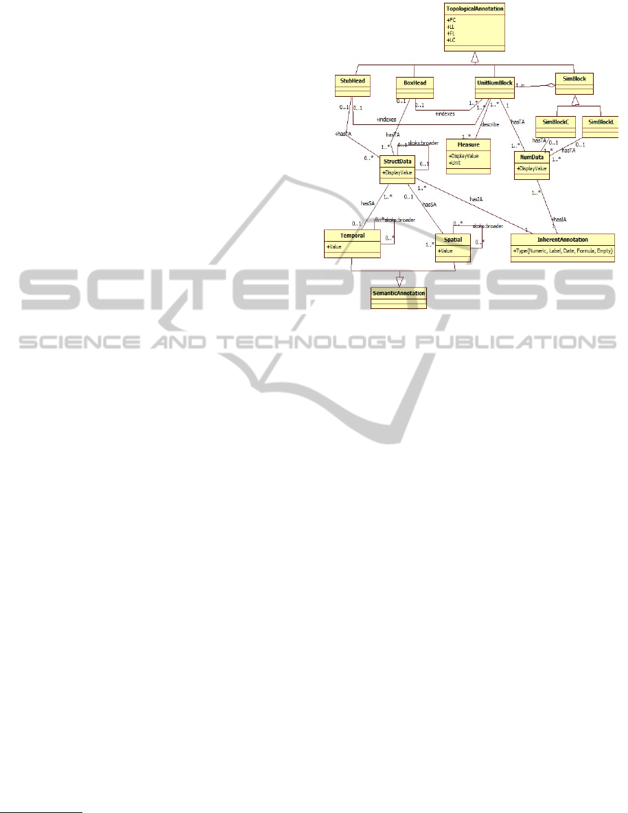
We propose, as depicted in Fig.2, a formalisation
of the ontology describing table annotations. We have
constructed this ontology manually. It forms a sup-
port for the automatic construction of each Open Data
source ontology as it will be detailed in the next sec-
tion. Each table is composed of two types of data:
(i) ”StructData” which means concepts (sequence of
words) able to express schema tables and (ii) ”Num-
Data” which means statistical or quantitative data.
For each data type, we associate three overlapping an-
notation types as follows:
• Inherent Annotation (IA) describes the low level
data types namely Numeric, Label, Formula and
Date.
• Topological Annotation (TA) describes name and
location of tables’ parts. As depicted in Fig.2,
the class ”TopologicalAnnotation” has four prop-
erties FL, LL, FC, LC (First Line, Last Line,
First Column, Last Column) representing respec-
tively the landmarks of the component in the ta-
ble. This class has different sub-classes: (i) ”Unit-
NumBlock” which is the body of table composed
ICEIS2015-17thInternationalConferenceonEnterpriseInformationSystems
272

Figure 3: The Workflow Activities Description.
it self by ”NumData” and describes a measure,
(ii) ”StubHead” and ”BoxHead” which are both
composed of ”StructData” and indexing ”Unit-
NumBlock” and (iii) ”SimBlock” composed of
”UnitNumBlock”. The ”SimBlock” has two sub-
classes: ”SimBlockC” (a block composed of Unit-
NumBlock indexed by the same StubHead and
different BoxHead) and ”SimBlockL” (a Block
composed of UnitNumBlock indexed by the same
BoxHead and different StubHead).
• Semantic Annotation (SA) describes the seman-
tic class of data, we focus on Temporal (Year,
Month,..) and Spatial (Region, GPS coordi-
nates,..) classes. The different types of concepts
will be related with a ”skos:broader”
3
relationship
to express the order between types.
2.2 The Workflow Activities Description
We propose, as depicted in Fig.3, a workflow activi-
ties transforming input flat open data (encapsulating
tables) into enrich annotated graphs. Each activity
will perform, in the same time, the table components
detection, ontology-guided annotation and graph con-
struction.
The first workflow activity consists of converting
flat open data into a matrix M which encodes low level
cells’ types namely Numeric, Label, Date and For-
mula. The vertices and relations for Inherent Annota-
tions are created in G
i
. Then, four activities, related to
search all types of blocks, are executed. The numer-
ical detection activity extracts all the UnitNumBlock,
creates in G
i
all the UnitNumBlock instances vertices
with their landmarks properties, creates NumData in-
stances vertices and finally makes relations (i.e anno-
tates) between each NumData and the UnitNumBlock
encapsulating it. The label (resp. date, formula) de-
tection activity extracts all blocks containing concepts
(resp. dates and formula) but does not add vertices
into G
i
.
3
http://www.w3.org/2009/08/skos-reference/skos.html
Thereafter, BoxHead and StubHead detection ac-
tivities use the detection results of numerical and
label activities. To identify the BoxHead (respec-
tively StubHead) of each UnitNumBlock, our algo-
rithm consists of a backtracking search of the first line
(respectively column) of labels situated above (re-
spectively on the left) the UnitNumBlock beginning
the search from the UnitNumBlock.FL (respectively
UnitNumBlock.FC). BoxHead, StubHead and Struct-
Data instances vertices contained into these blocks are
added to G
i
. Then the relationships between these lat-
ter are created into G
i
. Finally, indexing relationships
between UnitNumBlock, StubHead and BoxHead are
added into G
i
.
Similar block detection activity can be executed
after Stubhead or Boxhead activities. It groups dis-
joint UnitNumBlock having either the same BoxHead
(SimBlockC type) or the same StubHead (SimBlockL
type). Spatial detection activity uses the result of label
and numerical detections. It uses predefined lists
4
to
annotate instances present in the detected blocks. In
G
i
, the found instances are added and annotated with
their appropriate types. Hierarchical relationships are
expressed by the property skos:broder (a hierarchical
link indicating that a concept is more general than an-
other concept) between all spatial concepts.
Temporal detection uses date detection or numeri-
cal detection results. For temporal concepts, we refer
to the generic temporal graph defined by (Mansmann
and Scholl, 2007). We use regular expressions to
identify instances of each temporal entity. The mea-
sure detection activity uses the date detection and re-
lies on users to textually input measures names and
units.
The last activity is the hierarchical relationships
detection (skos:broader relations between StructData
as shown in Fig.2). Regarding the impact of com-
plex hierarchies (Malinowski and Zim
´
anyi, 2006) in
the summarizability problems, we focus on construct-
ing graphs with non complex hierarchies by applying
a set of rules (we will not detail them in this paper).
4
www.geonames.org
Graph-basedETLProcessesforWarehousingStatisticalOpenData
273

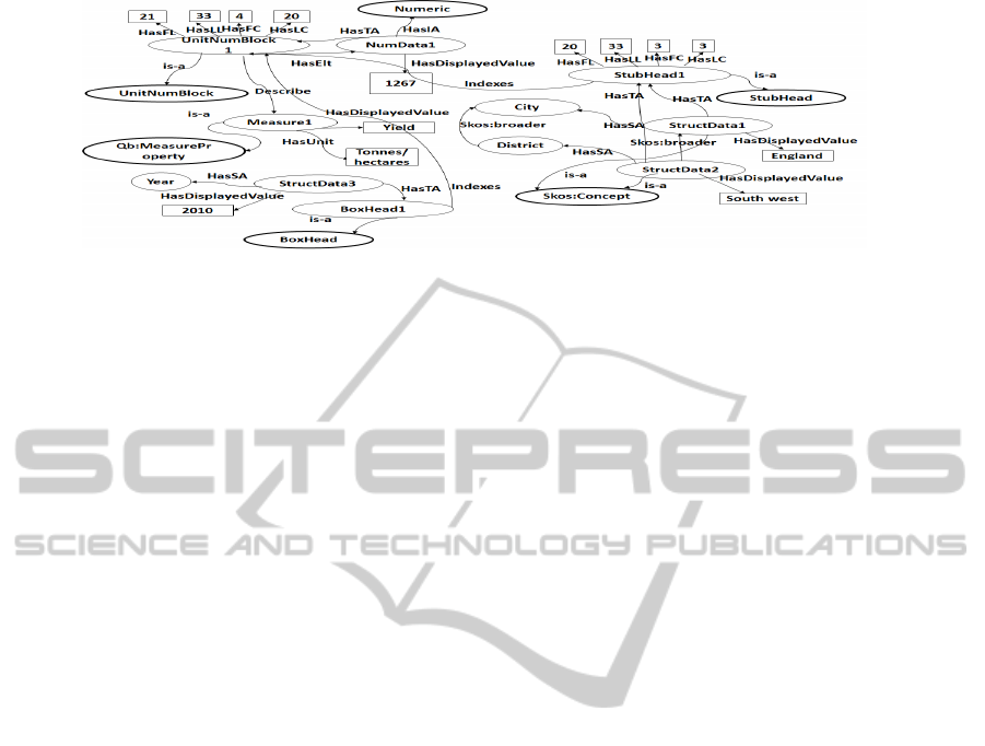
Figure 4: An excerpt from a resulting RDF Open Data Graph.
We propose two complementary alternatives for hier-
archical classification: (i) concept classification us-
ing annotations detected by the workflow activities
and (ii) concept classification using data mining tech-
niques to complement the first one. The first alter-
native is based on the arrangement of the numerical
blocks which can determine hierarchical relationships
between StubHead or BoxHead concepts. The second
alternative concerns Stubhead or Boxhead concepts.
We cross two conceptual classification techniques and
we select the relevant classes resulting from them.
The first technique is lattices (Birkhoff, 1967) which
does not consider semantic aspects and generates for-
mal contexts formed by concepts and attributes. The
second technique is RELEVANT (Bergamaschi et al.,
2011). It clusters a set of concepts and provide rele-
vant attributes for each cluster.
An Example of Open Data RDF Graph. An Open
Data Extraction Tool (ODET) has been implemented
to validate our approach (Berro et al., 2014). It per-
forms the workflow described above. Fig.4 repre-
sents an excerpt of the output graph resulting from
ODET for one source from our running example. This
source contains statistics on wheat production per
city, district and year. As depicted in Fig.4, the Unit-
NumBlock describes the yield measure which has as
unit Tonnes/Hectares. The StubHead is composed
of StructData, for instance we have StuctData1 with
value ”England” and StructData2 with value ”South
West”. StructData1 has the semantic annotation city
and StructData2 has the semantic annotation district.
The relation skos:broader between city and district
in the ontology has been instantiated in the instance-
schema graph between StructData1 and StructData2.
The BoxHead1, as an instance of the BoxHead class,
is the topological annotation of the StructData3 which
has as value 2010 and as semantic annotation Year.
3 HOLISTIC OPEN DATA GRAPH
INTEGRATION
This section is devoted to present our holistic inte-
gration approach based on the integer linear program-
ming technique.
3.1 Pre-matching Phase
This phase takes as input a set of N graphs G
i
=
(V
i
, E
i
) i ∈ [1, N], N ≥ 2 representing only struc-
tural schema elements which are StubHead, Box-
Head, spatio-temporal concepts and enrichment con-
cepts. The output of this phase is composed of: (1)
∑
N−1
i=1
(N − i) similarity matrices and (2) N direction
matrices representing the hierarchical relationships
between structural vertices.
Similarity Matrices Computation. We compute
∑
N−1
i=1
(N −i) similarity matrices denoted Sim
i, j
of size
n
i
× n
j
defined between two different graphs G
i
and
G
j
, ∀i ∈ [1, N − 1], j ∈ [i + 1, N]. Each matrix en-
codes similarity measures. We define the similarity
measure as the maximum between two known sim-
ilarity distances : (i) the syntactic measure Jaccard
(Jaccard, 1912) and (ii) the semantic measure Wup
(Wu and Palmer., 1994). As we deal with N input
graphs, similarity measure are computed between all
combination of all pairwise vertices concepts v
i
k
and
v
j
l
belonging to two different input graphs G
i
and G
j
such as i ∈ [1, N − 1], j ∈ [i + 1, N].
Sim
i, j
= {sim
i
k
, j
l
, ∀k ∈ [1, n
i
], ∀l ∈ [1, n
j
]}
Direction Matrices Computation. We compute a
set of N direction matrices Dir
i
of size n
i
× n
i
defined
for each graph G
i
, ∀i ∈ [1, N]. Each matrix encodes
edges directions and defined as follows:
ICEIS2015-17thInternationalConferenceonEnterpriseInformationSystems
274

Dir
i
={dir
i
k,l
, ∀k × l ∈ [1, n
i
] × [1, n
i
]}
dir
i
k,l
=



1 if e
i
k,l
∈ E
i
−1 if e
i
l,k
∈ E
i
0 otherwise
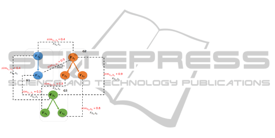
3.2 Matching Phase
The idea of the LP4HM matcher consist of extending
the maximum-weight graph matching problem with
additional logical implication constraints. These lat-
ter stand for constraints on matching setup and graph
structure. Fig.5 depicts three abstract graphs G
1
, G
2
and G
3
, and similarities between graph vertices (not
shown similarities are considered as null values).
Figure 5: An example of holistic graph matching problem.
Decision Variable. We define a single decision
variable which expresses the possibility to have or
not a matching between two vertices belonging to
two different input graphs. For each G
i
and G
j
,
∀i ∈ [1, N − 1], j ∈ [i + 1, N], x
i
k
, j
l
is a binary deci-
sion variable equals to 1 if the vertex v
i
k
in the graph
G
i
matches with the vertex v
j
l
in the graph G
j
and 0
otherwise.
Logical Implication Constraints. A logical impli-
cation (Plastria, 2002) is expressed as follows: for x
i
a binary variable for all i in some finite set I and y a
binary variable, if x
i
= 0 for all i ∈ I then y = 0 which
is also equivalent to y ≤
∑
i∈I
x
i
.
The first type of constraints belongs to Matching
Setup (MS). MS1 encodes the matching cardinality in
particular we focus on 1:1 matching (Rahm and Bern-
stein, 2001). MS2 encodes the matching threshold in
particular the model should not match vertices whose
similarity is inferior than a given threshold.
MS1 (Matching Cardinality.) Each vertex v
i
k
in the
graph G
i
could match with at most one vertex
v
j
l
in the graph G
j
, ∀i × j ∈ [1, N − 1] × [i +
1, N].
n
j
∑
l=1
x
i
k
, j
l
≤ 1, ∀k ∈ [1, n
i
]
MS2 (Matching Threshold.) We setup similarity
threshold thresh in order to get better match-
ing results. Our model encodes the threshold
setup in the following constraint : ∀i × j ∈
[1, N −1] × [i +1, N] and ∀k ×l ∈ [1, n
i
]×[1, n
j
]
sim
i
k
, j
l
x
i
k
, j
l
≥ thresh x
i
k
, j
l
The second type of constraints belongs to graph
structure. GS1 constraint generates strict hierarchies
and GS2 generates simple edge directions.
GS1 (Strict Hierarchies.) This constraint allow us
to resolve non-strict hierarchy problem (Mali-
nowski and Zim
´
anyi, 2006) which is an impor-
tant issue in multidimensional schema defini-
tion. Hence, users will save time in resolving
such problems in the multidimensional schema
definition step. ∀i × j ∈ [1, N − 1] × [i + 1, N]
and ∀k × l ∈ [1, n
i
] × [1, n
j
]:
x
i
k
, j
l
≤ x
i
pred(k)
, j
pred(l)
GS2 (Edge Direction.) The purpose of this constraint
is to prevent the generation of conflictual edges.
∀i × j ∈ [1, N − 1] × [i + 1, N] such as i 6= j and
∀k, k
0
∈ [1, n
i
] ∀l, l
0
∈ [1, n
j
]
x
i
k
, j
l
+ x
i
k
0
, j
l
0
+ (dir
i
k,k
0
dir
j
l,l
0
) ≤ 0
Objective Function. The objective of our model
is to maximize the sum of the similarities between
matched vertices. The objective function is expressed
as follows
N−1
∑
i=1
N
∑
j=i+1
n
i
∑
k=1
n
j
∑
l=1
sim
i
k
, j
l
x
i
k
, j
l
The resolution of the linear program of the exam-
ple in Fig.5 gives the following solution:
• v
1
2
matches with v
2
1
with sim
1
2
,2
1
= 0.9
• v
1
2
matches with v
3
1
with sim
1
2
,3
1
= 0.3
• v
2
1
matches with v
3
1
with sim
2
1
,3
1
= 0.9
• v
2
2
matches with v
3
2
with sim
2
2
,3
2
= 0.8
• v
2
3
matches with v
3
3
with sim
2
3
,3
3
= 0.8
• the objective function value is 3.7
Graph-basedETLProcessesforWarehousingStatisticalOpenData
275

4 INCREMENTAL DATA
WAREHOUSE SCHEMA
DEFINITION
In this section, we describe an incremental process to
define a multidimensional schema from the integrated
Open Data RDF graphs. The system will interact with
users’ actions in order to generate a script to create
the data warehouse schema and populate data, in the
same time the integrated RDF graph will be refined
with the QB4OLAP vocabulary proposed in (Etchev-
erry et al., 2014). QB4OLAP is more complete than
RDF Data Cube Vocabulary
5
(RDF QB) to describe
multidimensional schema. This twofold output is mo-
tivated by : (i) the interest of analysing populated data
with OLAP tools, (ii) the interest to keep reuse of in-
tegrated Open Data tables in other scenarios for in-
stance link them with available Statistical Open Data
or Linked Open Data in general.
4.1 A Conceptual Multidimensional
Schema and an Augmented RDF
Graph
Two types of output are expected from our incremen-
tal process. The outputs are described as follows :
A Conceptual Multidimensional Schema. We
will use the conceptual specifications of a generic
multidimensional schema (a group of star schema)
proposed in the works of (Ravat et al., 2008). This
generic model is the most suitable according to the al-
ternatives that can generate the integrated graph (for
instance several facts which share the same dimen-
sions). A multidimensional schema E is defined by
(F
E
, D
E
, Star
E
) such as :
• F
E
= {F
1
, . . . , F
n
} a finite set of facts;
• D
E
= {D
1
, . . . , D
m
} a finite set of dimensions;
• Star
E
: F
E
→ 2
DE
a function associating for each
fact a set of dimensions.
A dimension D ∈ D
E
is defined by (N
D
, A
D
, H
D
):
• N
D
a dimension name,
• A
D
= {a
D
1
, . . . , a
D
u
} ∪ {id
D
, All} a set of attributes,
• H
D
= {H
D
1
, . . . , H
D
v
} a set of hierarchies.
A hierarchy denoted H
i
∈ H
D
is defined by (N
H
i
,
Param
H
i
, Weak
H
i
) such as:
• N
H
i
a hierarchy name,
5
http://www.w3.org/TR/vocab-data-cube/
• Param
H
i
= < id
D
, p
H
i
1
, . . . , p
H
i
v
i
, All > an ordered
set of attributes called parameters which repre-
sent the relevant dimension’ graduations, ∀k ∈
[1. . . v
i
], p
H
i
k
∈ A
D
,
• Weak
H
i
: Param
H
i
→ 2
A
D
−Param
H
i
is a function as-
sociating each parameter to one or several weak
attribute.
A fact denoted F ∈ F
E
is defined by (N
F
, M
F
):
• N
F
a fact name,
• M
F
= f
1
(m
F
1
), . . . , f
w
(m
F
w
) a set of measures asso-
ciated to an aggregation function f
i
.
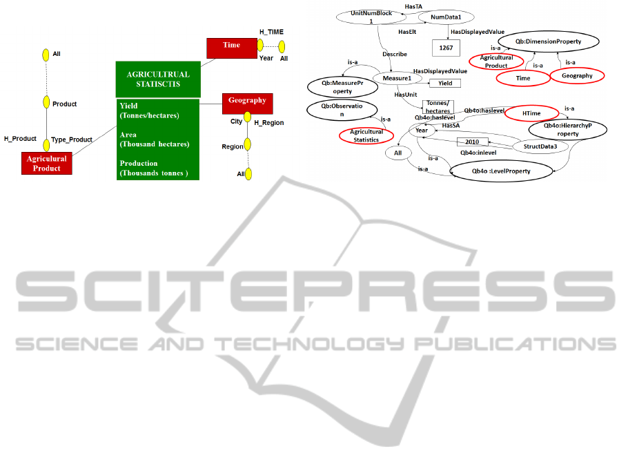
Example 1. The example depicted in Fig.6(a) is
the expected multidimensional schema from the
phase 3 of our process applied to the motivat-
ing example. For the sake of simplicity, fact
F
i
, dimension D
i
and hierarchy H
i
are cited by
their names. The multidimensional schema E
is composed of one fact and three dimensions.
E = ({AgriculturalStatistics}, {Time, Geography,
AgriculturalProduct}, {Star(AgriculturalStatistics)=
{Time, Geography, AgriculturalProduct} ) The di-
mensions are : (Time, {Year, All}, {HTime}),
(Geography, {City, Region, All}, {HRegion})
and (AgriculturalProduct, {TypeProduct, Product ,
All}, {HProduct}). The fact is : (Agricultural-
Statistics, {AVG(Yield), SUM(Area), AVG(Area),
SUM(Production), AVG(Production)})
An Augmented RDF Graph. The integrated RDF
graph resulting from the matching phase will be aug-
mented with concepts belonging to the QB4OLAP
vocabulary proposed in (Etcheverry et al., 2014). This
latter uses the basic concepts of RDF QB and extends
it with concepts representing hierarchies, hierarchies
levels, aggregation functions, cardinalities. The cor-
respondences between the multidimensional schema
and the concepts of the RDF graph are as follows:
• E is an instance of qb : dataStructureDe f inition.
• F
E
is an instance of a qb : Observation class.
• D
E
is an instance of a qb : DimensionProperty
class.
• Star
E
: F
E
→ 2
DE
is an instance of qb : DataSet.
• A
D
is an instance of qb4o : levelProperty
• The members of A
D
are instances of qb :
leveMumber.
• H
D
is an instance of qb4o : HierarchyProperty.
• Param
H
i
is an instance of qb4o : LevelProperty.
• Weak
H
i
is an instance of a qb : AttributeProperty.
ICEIS2015-17thInternationalConferenceonEnterpriseInformationSystems
276

(a) An example of Multidimensional Schema (b) An Augmented RDF Graph
Figure 6: Expected outputs for the incremental schema definition step.
• M
F
is an instance of qb : MeasureProperty and
the associated aggregation function f
i
is an in-
stance of qb4o : AggregateFunction.
The Fig.6(b) shows an excerpt of an expected aug-
mented RDF graph by following the correspondences
explained above.
The processes we use to obtain the two expected
results will be explained in the next section.
4.2 An Incremental Process to Define
Multidimensional Components
We propose an incremental process in which users
should begin by identifying dimensions and their
components (hierarchies, attributes, members) then
they define the fact and its measures. Three ac-
tors interact in this process: (1) users who interact
with the integrated graph via different functions to in-
crementally define multidimensional components, (2)
graph transformation (GT) which interacts with user’
actions in order to enrich the integrated graph with
OLAP4QB objects and properties, (3) data warehouse
script generator (SG) which interacts with user’ ac-
tions in order to generate the script describing the
multidimensional schema and from which the data
warehouse will be populated with SOD.
Dimensions Identification. When a user
add dimensions, the GT creates a new vertex
with the dimension name as an instance of a
qb:dimensionProperty and the SG creates a new
table dimension without attributes. Then user add
hierarchies to the dimension, but as hierarchies are
composed of levels, users have to choose either
to add level or to select a level from the graph.
If user chooses the action add level, the GT cre-
ates a vertex with the hierarchy name instance
of qb4o:hierarchyProperty, a vertex for the level
instance of qb4o:levelProperty and a property
qb4o:haslevel between the hierarchy and the level. If
the user chooses the action select level form graph,
this level had to be a StructData vertex, it will be
changed to become an instance of qb4o:levelProperty
and the property qb4o:haslevel will be created
between this vertex and the hierarchy level. Then for
both actions add level and select level from graph,
user have to select members form the graph. The
GT will collect members from graph which are
StructData. These members are changed into in-
stances of qb:levelMemeber. Properties qb4o:inlevel
will be created between the concerned level and its
members and visually these vertices will be collapsed
in the label vertex. In the same time, the SG updates
dimension with its attributes, creates hierarchies with
levels and populates dimension attributes with their
members. The users have to iterate the described
process for all dimensions knowing that when a
the task of dimension creation finish, the system
can suggest to user potential dimensions. Indeed,
since each NumData is related to a path composed
of a succession of StructData, the GT deduces the
NumData related to the paths belonging to the actual
identified dimension and proposes to the users the
non yet identified paths related to the NumData as a
potential dimension.
Fact Identification. When all dimensions have
been identified, the user can proceed to fact and mea-
sures identification. When the user creates a fact, the
GT creates a vertex with the fact name as an instance
of qb:observation. Then he should link dimensions to
the fact, and select measures from the graph. So, the
SG creates a fact table with its measures and relates
it to the created dimensions. GT collects the Num-
Data related to the selected dimensions and measures
which are instances of the qb:dataset. Finally SG add
these instances to the fact table.
Graph-basedETLProcessesforWarehousingStatisticalOpenData
277

Discussion and Future Work. In the process de-
scribed above, the user intervention can be error-
prone hence some improvements may be envisaged.
For instance, we can inject some of the algorithms
proposed by (Romero and Abell
´
o, 2007) in order to
semi-automate the identification of dimensions and
facts. Moreover, even if we have resolved the prob-
lem of complex hierarchies in the first two steps of our
ETL processes by generating strict hierarchies, we ac-
knowledge that the summarizabiliy problem (Maz
´
on
et al., 2010) is not totally resolved especially com-
pleteness and disjointness integrity constraints (Lenz
and Shoshani, 1997). Both the works of (Romero and
Abell
´
o, 2007) and (Prat et al., 2012) propose solu-
tions applied on ontologies. Compared to (Romero
and Abell
´
o, 2007), the authors of (Prat et al., 2012)
propose more explicit rules which seems straightfor-
ward to be added to our process. Since the construc-
tion of our process outputs are performed in paral-
lel, the verification of the summarizabilty constraints
in the ontology will be used to check the same con-
straints in the multidimensional model.
5 CONCLUSIONS
In this paper, we have presented a full RDF graph-
based ETL chain for warehousing SOD. This ETL
chain takes as input a set of flat SOD containing sta-
tistical tables and transforms them into a multidimen-
sional schema through three steps. The first step au-
tomatically extracts, annotates and transforms input
tables into RDF instance-schema graphs. The second
step performs automatically a holistic graph integra-
tion through an integer linear program. The third one
incrementally defines the multidimensional schema
through an interactive process between users and sys-
tem. The main contributions of our approach are:
(i) the unified representation of tables which facili-
tates their schema discovery and (ii) the extension of
the maximum weighted graph matching problem with
structural constraints in order to resolve the holistic
open data integration problem. In our future works,
we aim to train a user study on our approach to mea-
sure the efficiency of automatic detections and inte-
grations, and to measure the difficulties that users may
encounter when they define incrementally the multi-
dimensional schema from visual graphs.
REFERENCES
Bergamaschi, S., Guerra, F., Orsini, M., Sartori, C., and
Vincini, M. (2011). A semantic approach to etl
technologies. Data and Knowledge Engineering,
70(8):717 – 731.
Berro, A., Megdiche, I., and Teste, O. (2014). A content-
driven ETL processes for open data. In New Trends in
Database and Information Systems II - Selected pa-
pers of the 18th East European Conference on Ad-
vances in Databases and Information Systems and As-
sociated Satellite Events, ADBIS 2014 Ohrid, Mace-
donia, pages 29–40.
Birkhoff, G. (1967). Lattice Theory. American Mathemati-
cal Society, 3rd edition.
Etcheverry, L., Vaisman, A., and Zimnyi, E. (2014). Mod-
eling and querying data warehouses on the semantic
web using QB4OLAP. In Proceedings of the 16th
International Conference on Data Warehousing and
Knowledge Discovery, DaWaK’14, Lecture Notes in
Computer Science. Springer-Verlag.
Jaccard, P. (1912). The distribution of the flora in the alpine
zone. New Phytologist, 11(2):37–50.
Lenz, H.-J. and Shoshani, A. (1997). Summarizability in
olap and statistical data bases. In Scientific and Sta-
tistical Database Management, 1997. Proceedings.,
pages 132–143.
Malinowski, E. and Zim
´
anyi, E. (2006). Hierarchies in
a multidimensional model: From conceptual mod-
eling to logical representation. Data Knowl. Eng.,
59(2):348–377.
Mansmann, S. and Scholl, M. H. (2007). Empowering the
olap technology to support complex dimension hierar-
chies. IJDWM, 3(4):31–50.
Maz
´
on, J.-N., Lechtenbrger, J., and Trujillo, J. (2010). A
survey on summarizability issues in multidimensional
modeling. In JISBD, pages 327–327. IBERGARC-
ETA Pub. S.L.
Plastria, F. (2002). Formulating logical implications in com-
binatorial optimisation. European Journal of Opera-
tional Research, 140(2):338 – 353.
Prat, N., Megdiche, I., and Akoka, J. (2012). Multidi-
mensional models meet the semantic web: defining
and reasoning on OWL-DL ontologies for OLAP. In
DOLAP 2012, ACM 15th International Workshop on
Data Warehousing and OLAP, pages 17–24.
Rahm, E. and Bernstein, P. A. (2001). A survey of
approaches to automatic schema matching. VLDB
JOURNAL, 10.
Ravat, F., Teste, O., Tournier, R., and Zurfluh, G. (2008).
Algebraic and graphic languages for OLAP manipu-
lations. International Journal of Data Warehousing
and Mining, 4(1):17–46.
Romero, O. and Abell
´
o, A. (2007). Automating multidi-
mensional design from ontologies. In Proceedings of
the ACM Tenth International Workshop on Data Ware-
housing and OLAP, DOLAP ’07, pages 1–8. ACM.
Wang, X. (1996). Tabular abstraction, editing, and format-
ting. Technical report, University of Waretloo, Water-
loo, Ontaria, Canada.
Wu, Z. and Palmer., M. (1994). Verb semantics and lexical
selection. In In 32nd. Annual Meeting of the Associa-
tion for Computational Linguistics, New Mexico State
University, Las Cruces, New Mexico., pages 133–138.
ICEIS2015-17thInternationalConferenceonEnterpriseInformationSystems
278