
Fuzzy Resource Allocation Mechanisms in Workflow Nets
Joslaine Cristina Jeske de Freitas, St´ephane Julia and Leiliane Pereira de Rezende
Computer Science, Federal University of Uberlˆandia,
Av. Jo˜ao Naves de
´
Avila, 2121, 38400-902, Uberlˆandia, Minas Gerais, Brazil
Keywords:
Petri Net, Workflow Net, Resource Allocation, Fuzzy Time, Possibility Theory.
Abstract:
The purpose of Workflow Management Systems is to execute Workflow processes. Workflow processes rep-
resent the sequence of activities that have to be executed within an organization to treat specific cases and to
reach a well-defined goal. Therefore, it is to manage in the best possible way time and resources. The proposal
of this work is to express in a more realistic way the resource allocation mechanisms when human behavior is
considered in Workflow activities. In order to accomplish this, fuzzy sets delimited by possibility distributions
will be associated with the Petri net models that represent human type resource allocation mechanisms. Addi-
tionally, the duration of activities that appear on the routes (control structure) of the Workflow process, will be
represented by fuzzy time intervals produced through a kind of constraint propagation mechanism. New firing
rules based on a joint possibility distribution will then be defined.
1 INTRODUCTION
The purpose of Workflow Management Systems is
to execute Workflow processes. Workflow processes
represent the sequence of activities that have to be ex-
ecuted within an organization to treat specific cases
and to reach a well-defined goal. Of all notations used
for the modeling of Workflow processes, Petri nets
are very suitable (van der Aalst and van Hee, 2004),
as they represent basic routings. Moreover, Petri nets
can be used for specifying the real time characteris-
tics of Workflow Management Systems (in the time
Petri net case) as well as complex resource allocation
mechanisms. As a matter of fact, late deliveries in an
organization are generally due to resources overload.
Many papers have already considered the Petri net
theory as an efficient tool for the modeling and anal-
ysis of Workflow Management Systems. In (van der
Aalst and van Hee, 2004), Workflow nets, which are
acyclic Petri net models used to represent Workflow
process, are defined.
Workflow nets have been identified and widely
used as a solid model of Workflow processes, for
example in (Aalst, 1997), (van Hee et al., 2006),
(Martos-Salgado and Rosa-Velardo, 2011), (Wang
and Li, 2013). In (Ling and Schmidt, 2000), an ex-
tension of Workflow nets is presented. This model
is called time Workflow net and associates time inter-
vals with the transitions of the correspondingPetri net
model. In (Kotb and Badreddin, 2005), an extended
Workflow Petri net model is defined. Such a model
allows for the treatment of critical resources which
have to be used for specific activities in real time. In
(Wang et al., 2009), a resource-oriented Workflow net
(ROWN) based on a two-transition task model was
introduced for resource-constrained Workflow mod-
eling and analysis. Considering the possibility of task
failure during execution, in (Wang and Li, 2013), a
three-transition task model to specify a task start, end
and failure was proposed. Additional research can be
found in (Adoglaand Collins, 2014), (He et al., 2014),
(Deng et al., 2014) and (Guo et al., 2014).
The majority of existing models put their focus
on the process aspect and do not consider important
characteristics of the Workflow Management System.
In (Aalst, 1997) and (van Hee et al., 2006) for ex-
ample, the resource allocation mechanisms are repre-
sented only in an informal way. In (Ling and Schmidt,
2000), (Kotb and Badreddin, 2005) and (Wang and
Li, 2013) resource allocation mechanisms are repre-
sented by simple tokens in places as it is generally the
case in production systems (Lee and DiCesare, 1994).
But a simple token in a place will not represent in a
realistic way humanemployees who can treat simulta-
neously different cases in a single day, as it is usually
the case in most Business processes.
The proposal of this work is to express in a more
realistic way resource allocation mechanisms when
471
Cristina Jeske de Freitas J., Julia S. and Pereira de Rezende L..
Fuzzy Resource Allocation Mechanisms in Workflow Nets.
DOI: 10.5220/0005365304710478
In Proceedings of the 17th International Conference on Enterprise Information Systems (ICEIS-2015), pages 471-478
ISBN: 978-989-758-096-3
Copyright
c
2015 SCITEPRESS (Science and Technology Publications, Lda.)
human behavior is considered. For that, fuzzy sets de-
limited by possibility distributions (Duboisand Prade,
1988) will be associated with the Petri net models that
represent human type resource allocation mechanisms
and fuzzy time intervals will be associated to activity
durations. A firing mechanism using a joint possi-
bility distribution will then be defined in order to as-
sociate through a single formalism explicit time con-
straints as well as resource availability information.
The remainder of this paper is as follows. Section
2 introduces the concepts of fuzzy sets and possibil-
ity measures. Section 3 shows Workflow modeling.
Section 4 presents resource allocation mechanisms.
Section 5 presents a fuzzy time constraint propaga-
tion mechanism. Section 6 defines new firing rules
that consider fuzzy time constraints as well as fuzzy
resource allocation mechanisms. Finally, section 7
concludes the paper and provides references for ad-
ditional works.
2 FUZZY SETS AND
POSSIBILITY MEASURES
The notion of fuzzy set was introduced by (Zadeh,
1965) in order to represent the gradual nature of hu-
man knowledge. For example, the size of a man
could be considered by the majority of a population
as small, normal, tall, etc. A certain degree of belief
can be attached to each possible interpretationof sym-
bolic information and can simply be formalized by a
fuzzy set F of a reference set X that can be defined by
a membership function µ
F
(x) ∈ [0, 1]. In particular,
for a given element x ∈ X, µ
F
(x) = 0 denote that x is
not a member of the set F, µ
F
(x) = 1 denotes that x is
definitely a member of the set F, and intermediate val-
ues denote the fact that x is more or less an element of
F. Normally, a fuzzy set is represented by a trapezoid
A = [a1, a2, a3, a4] as the one represented in figure 1
where the smallest subset corresponding to the mem-
bership value equal to 1 is called the core, and the
largest subset corresponding to the membership value
greater than 0 is called the support.
Figure 1: Representation of a fuzzy set.
There exist three particular cases of fuzzy sets that
are generally considered:
• the triangular form where a2=a3,
• the imprecise case where a1=a2 and a3=a4,
• the precise case where a1=a2=a3=a4.
When considering two distincts fuzzy sets A and
B, the basic operations are as follows (Klir and Yuan,
1995):
• the fuzzy sum A⊕ B defined as:
[a1, a2, a3, a4] ⊕ [b1, b2, b3, b4] =
[a1+ b1, a2+ b2, a3+ b3, a4+ b4],
• the fuzzy subtraction A⊖ B defined as:
[a1, a2, a3, a4] ⊖ [b1, b2, b3, b4] =
[a1− b4, a2− b3, a3− b2, a4− b1],
• the fuzzy product A⊗ B defined as:
[a1, a2, a3, a4] ⊗ [b1, b2, b3, b4] =
[a1.b1, a2.b2, a3.b3, a4.b4].
A fuzzy set F can be delimited by a possibility dis-
tribution Π
f
, such as: ∀x ∈ X, Π
f
(x) = µ
F
(x) (Dubois
and Prade, 1988),(Cardoso et al., 1999). Given a pos-
sibility distribution Π
a
(x), the measure of possibility
Π(S) and necessity N(S) that a data a belongs to a
crisp set S of X is defined by Π(S) = sup
x∈S
Π
a
(x) and
N(S) = inf
x6∈S
(1− Π
a
(x)) = 1 − Π(
S). If Π(S) = 0,
it is impossible that a belongs to S. If Π(S) = 1, it is
possible that a belongs to S, but it also depends on the
value of N(S). If N(S) = 1, it is certain that (the larger
the value of N(S), the more the propositionis believed
in). In particular, there exists a duality relationship
between the modalities of the possible and the neces-
sary which postulates that an event is necessary when
its contrary is impossible. Some practical examples
of possibility and necessity measures are presented in
(Dubois and Prade, 1988).
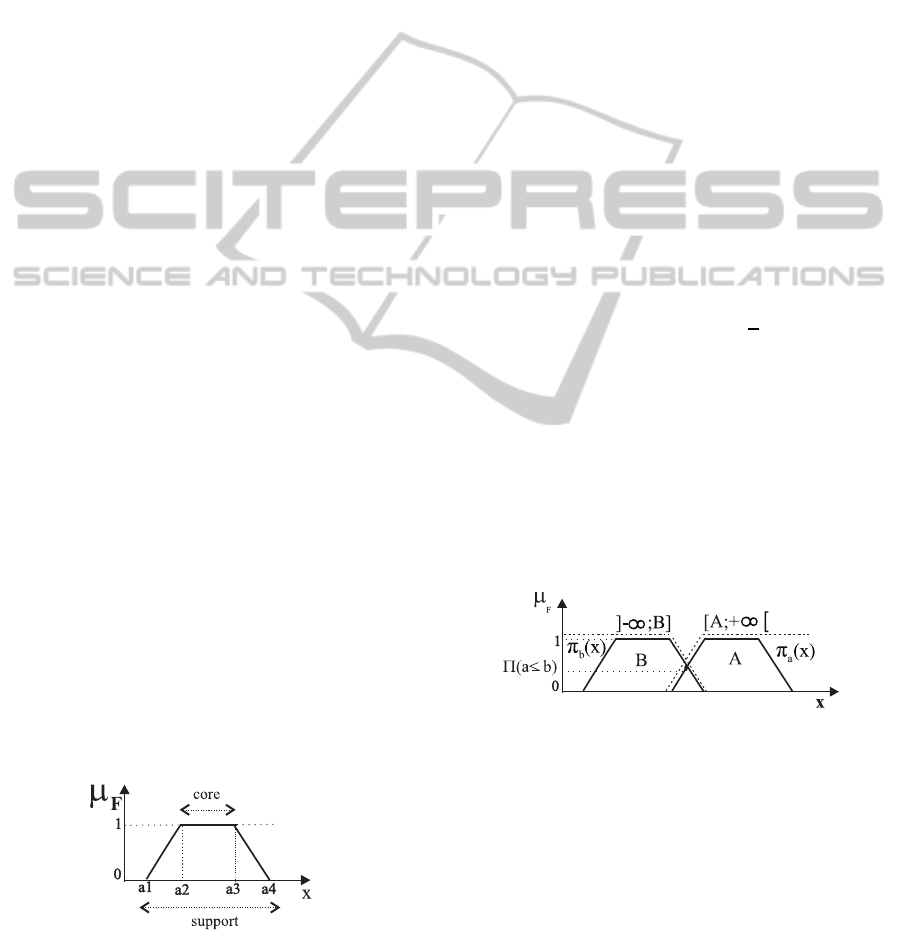
Figure 2: Possibility Measure.
Given two data a and b characterized by two fuzzy
sets A and B as shown in figure 2, the measure of pos-
sibility and necessity of having a ≤ b are defined as:
Π(a ≤ b) = sup
x≤y
(min(Π
a
(x), min(Π
b
(y))) =
max([A, +∞[∩] − ∞, B]) (1)
and
N(a ≤ b) = 1− sup
x≤y
(min(Π
a
(x), min(Π
b
(y))).
(2)
ICEIS2015-17thInternationalConferenceonEnterpriseInformationSystems
472

Given a normalized possibility distribution π
a
,
(Dubois and Prade, 1989) defines the following fuzzy
sets of the time point that are:
• possibly after a: µ
[A,+∞[
(x) = sup
x∈X
π
a
(s) (see
figure 3);
• necessarily after a: µ
]A,+∞[
(x) = in f
x∈X
(1− π
a
(s))
(see figure 3);
• possibly before a: µ
]−∞,A]
(x) = sup
x∈X
π
a
(s) (see
figure 4);
• necessarily before a: µ
]−∞,A[
(x) = inf
x∈X
(1 −
π
a
(s)) (see figure 4).
1
0
X
A
[A,+ [¥
]A,+ [¥
Figure 3: Possibly/necessarily after a.
1
0
X
A
]- ,A]¥
]- ,A[¥
Figure 4: Possibly/necessarily before a.
A visibility time interval [a, b] is a period of time
between two dates a and b. In the case where a and
b are fuzzy dates A and B (delimited by π
a
and π
b
)
respectively, the interval [a, b] is represented by the
the following pair of fuzzy sets:
• [A, B], the conjunctive set of time instants that rep-
resents the set of dates possibly after A and possi-
bly before B;
• ]A, B[, the conjunctive set of time instants that rep-
resents the set of dates necessarily afterA and nec-
essarily before B.
The joint possibility admits as upper bound in
(Dubois and Prade, 1988):
∀x ∈ X ∀y ∈ Y π(x, y) = min(π
X
(x), π
Y
(y)) (3)
when the reference sets are non-interactive (the value
of x in X has no influence on the value of y in Y, and
vice versa).
3 WORKFLOW MODELING
Modeling a Workflow process in terms of a Workflow
net is rather straightforward: transitions are active
components and models the tasks, places are passive
components and model conditions (pre and post), and
tokens model the cases to be treated (van der Aalst
and van Hee, 2004).
To illustrate the mapping of a process into a Work-
flow net, the process for handling complaints, shown
in (van der Aalst and van Hee, 2004) is considered: an
incoming complaint is first recorded. Then the client
who has complained along with the department af-
fected by the complaint are contacted. The client is
approached for more information. The department is
informed of the complaint and may be asked for its
initial reaction. These two tasks may be performed
in parallel, i.e. simultaneously or in any order. After
this, data is gathered and a decision is made. Depend-
ing upon the decision, either a compensation payment
is made or a letter is sent. Finally, the complaint is
filed. In Figure 5, a Workflow net that correctly mod-
els this process is shown.
W5
W3
W7
A2(Contact Client)
W4
W2
W1
A6 (Pay)
Start
A1 (Record)
A3(Contact_Department)
A4(Collect)
A5(Assess)
A7(Send_Letter)
A8 (File)
End
W6
Figure 5: “Handle Complaint Process”.
As mentioned previously, a task can be associated
to a transition in a Workflow net. However, in order to
catch resources in use when a task is in execution and
released them when the task is done, we use two se-
quential transitions plus a place to model a task. The
first transition representsthe beginningof the task, the
place the task, and the second transition the end of the
task (Wang et al., 2009).
FuzzyResourceAllocationMechanismsinWorkflowNets
473

A3A3
A3
B
E
Figure 6: Petri net model of a task.
As shown in figure 6, transition B represents the
beginning of a task execution; E represents the end
of the task execution. Place A3 represents the task
in execution. From reachability analysis perspective,
figure 6 can be reduced to a single transition which
represents the entire task execution as a single logic
unit.
4 RESOURCE ALLOCATION
MECHANISM
Resources in Workflow Management Systems are
non-preemptive (van der Aalst and van Hee, 2004):
once a resource has been allocated to a specific activ-
ity, it cannot be free before ending the corresponding
activity. As already mentioned, there exists different
kinds of resources in Workflow processes. Some of
which are of the discrete type and can be represented
by a simple token. For example, a printer used to treat
a specific class of documents will be represented as
a non-preemptive resource and could be allocated to
a single document at a same time. On the contrary,
some other resources cannot be represented by sim-
ple tokens. This is generally the case with human
type resources. As a matter of fact, it is not unusual
for an employee who works in an administration to
treat several cases simultaneously. For example, in an
insurance company, a single employee can normally
treat several documents during a working day and not
necessarily in a pure sequential order. In this case,
a simple token could not model human behavior in a
proper manner.
[100,100,
100,100]
[20,30,30,40]
[20,30,30,40]
[40,50,50,60]
[40,50,50,60]
[30,40,40,50]
[30,40,40,50]
[1,1,1,1]
[1,1,1,1]
[1,1,1,1]
[1,1,1,1]
[1,1,1,1]
[1,1,1,1]
B-A3
E-A3
B-A2
E-A2
B-A7
E-A7
RFC
Employee-
Complaints
A3
(Contact-
Cliente)
A2
(Contact-
Department)
A7
(Send-
Letter)
Figure 7: Fuzzy Continuous Resource.
Fuzzy allocation mechanisms were presented in
(Jeske et al., 2009). An example of fuzzy continuous
resource is given in figure 7. For example, this fig-
ure shows that 30%± 10% of the resource availabil-
ity R2 is necessary to realize the activity A3 (Contact-
Client).
The behavior of a fuzzy continuous resource allo-
cation model can be defined through the concepts of
“enabled transition” and “fundamental equation”.
In an ordinary Petri net, a transition t is enabled
if and only if for all the input places p of the transi-
tion, M(p) ≥ Pre(p, t), which means that the number
of tokens in each input place is greater or equal to the
weight associated to the arcs which connect the input
places to the transition t. With a fuzzy continuous re-
source allocation mechanism, considering a transition
t, the marking of an input place p and the weights as-
sociated to the arc which connects this place to the
transition t are defined through different fuzzy sets.
In this case, a transition t is enabled if and only if (for
all the input places of the transition t):
Π
t
= Π(Pre
FCR
(p,t) ≤ M
FCR
(p)) > 0. (4)
Figure 8: Possibility Measure of B-A3.
For example, the transition B-A3 in figure 7 is
enabled because Π
B−A3
= Π(Pre
FCR
(R2,B−A3) ≤
M
FCR
(R2)) = 1 > 0 as shown in figure 8 (a =
Pre
FCR
(R2,B−A3) and b = M
FCR
(R2)).
For an ordinary Petri net, once a transition is en-
abled by a marking M, it can be fired and a new mark-
ing M
′
is obtained according to the fundamentalequa-
tion:
M
′
(p) = M(p) − Pre(p, t) + Pos(p, t). (5)
With a fuzzy continuous resource allocation
model, the marking evolution is defined through the
following fundamental equation:
M
′
FCR
(p) = M
FCR
(p) ⊖ Pre
FCR
(p,t) ⊞ Pos
FCR
(p,t)
(6)
The operation “⊖” corresponds to the fuzzy sub-
traction. The operation “⊞”, when considering the
sum of two fuzzy sets, is different from the one given
in fuzzy logic and is defined as:
[a1, a2, a3, a4] ⊞ [b1,b2,b3, b4] =
[a1+ b1, a2+ b2, a3+b3, a4+b4].
This difference is due to the fact that the fuzzy
operation “⊕” does not maintain the marking of the
ICEIS2015-17thInternationalConferenceonEnterpriseInformationSystems
474

fuzzy continuous resource allocation model invariant
(the p-invariant property of the Petri net theory (Mu-
rata, 1989)). As a matter of fact, after realizing differ-
ent activities, the resource’s availability must go back
to 100 %, even in the fuzzy case. To a certain extent,
from the point of view of fuzzy continuous resource
allocation mechanisms, the operation “⊞” can be seen
as a kind of defuzzyfication operation. In particular,
using this operation, it will be possible to find a linear
expression of the fuzzy marking which will always be
constant and which will correspond to the following
expression:
M
FCR
(R
FC
) ⊞ (w
1
⊗ M
FCR
(A1)) ⊞ (w
2
⊗M
FCR
(A2)) ⊞ ·· · ⊞ (w
N
FCR
⊗
M
FCR
(A
N
FCR
)) = CONST. (7)
with w
α
= Pre
FCR
(R
FC
,t
in
α
) = Pos
FCR
(R
FC
,t
out
α
)
for α = 1 to N
FCR
.
5 FUZZY TIME CONSTRAINT
PROPAGATION MECHANISM
As the actual time required by an activity in a Work-
flow Management System is non-deterministic and
not easily predicted, a fuzzy time interval can be as-
signed to every Workflow activity.
The static definition of a fuzzy time Workflow
net is based on fuzzy static intervals [a1,a2, a3, a4]s
which represent the permanency duration (sojourn
time) of a token in places. Before duration a1 the
token is in the non-available state. After a1 and be-
fore a4, the token is in the available state for the fir-
ing of a transition. After a4, the token is again in the
non-available state and cannot enable any transition:
it therefore becomes a dead token. In a real time sys-
tem case, the “death” of a token has to be seen as a
time constraint that is not respected. A transition can-
not be fired with dead tokens as this would correspond
to an illegal action or behavior: a constraint violation.
The dynamic evolution depends on the time situation
of the tokens (date intervals associated with the to-
kens). For example, if the arrival date of the token in
the place is δ = 3, knowing that the fuzzy static inter-
val of this place is [5, 6, 7,8]v, then, the fuzzy visibil-
ity interval of this token is [5+3, 6+3, 7+3, 8+3]v=
[8, 9, 10, 11]v.
In a Workflow Management System, a visibility
interval depends on a global clock associated to the
entire net which calculates the passage of time from
date = 0, which corresponds to the start of the sys-
tems operation. In particular, the existing waiting
B-A4
B-A1
E-A4
A3
(Contact-Department)
[20,25,35,40]s
A6(Pay)
[0,5,15,20]s
B-A5
E-A1
B-A3
B-A2
E-A3
E-A2
E-A5
B-A6
B-A7
E-A6
E-A7
B-A8
E-A5
E-A8
R2
(Employee-Complaints)
[0, [s
R4(Assessor-
Complaints)
[0, [s
R3(System)
[0, [s
R5
(Employee
Finances)
[0, [s
R1( Secretary)
[0, [s
A1 (Record)
[0,5,10,15]s
A2
(Contact-Client)
[15,20,30,35]s
A4(Collect)
[0,0,0,0]s
A5(Assess)
[10,15,25,30]s
A7(Send-Letter)
[15,20,30,35]s
A8(File)
[0,0,0,0]s
[100,100,100,
100]
[30,40,40,50]
[30,40,40,50]
[20,30,30,40]
[20,30,30,40]
[40,50,50,60]
[40,50,50,60]
Start
[0,5,25,50]v
W2
[0,10,35,55]v
W1
[0,10,40,60]v
W4
[20,35,70,85]v
W3
[15,30,70,85]v
W5
[20,35,70,85]v
W6
[30,50,95,105]v
W7
[30,50,95,105]v
W8
[30,50,95,105]v
W9
[45,70,110,115]v
End
[45,70,110,115]v
8
8
8
8
8
t
[100,100,100,
100]
[100,100,100,100]
[100,100,100,100]
[100,100,100,
100]
[100,100,100,100]
[100,100,100,100]
[100,100,100,100]
[100,100,100,
100]
[100,100,100,100]
[100,100,100,100]
Figure 9: Visibility intervals of the “Handle Complaint Pro-
cess”.
times between sequential activities can be represented
by visibility intervals whose minimum and maximum
fuzzy boundaries will depend on the earliest and lat-
est delivery dates of the considered case. Through
correct knowledge of the beginning date of the pro-
cess and the maximum duration of a case, it is pos-
sible to calculate estimated visibility intervals associ-
ated with each token in each waiting place using con-
straint propagationtechniques very similar to the ones
used in scheduling problems based on activity-on-arc
graphs without circuits (Gondran et al., 1984).
Figure 9 shows the fuzzy static intervals (intervals
of fuzzy durations) associated to the activity places
of the process and the fuzzy visibility intervals (inter-
vals of fuzzy dates) associated with the waiting places
(condition places of the workflow net). It is important
to note that there is no time restriction on resources -
static interval defined for each resource is [0, ∞[s. The
minimal fuzzy bounds of the estimated visibility in-
tervals attached to the waiting places are calculated
applying a forward constraint propagation technique
applied to the different kinds of routings associated
with the “Handle Complaint Process”, and the max-
imum fuzzy bounds of the estimated visibility inter-
FuzzyResourceAllocationMechanismsinWorkflowNets
475

vals are calculated by applying a backward constraint
propagation techniques to the different kinds of rout-
ings considering the latest delivery dates of the case.
If the token appears in a place p at date δ and if its
visibility interval is given by [a1, a2, a3, a4], then this
token could be used for the firing of a transition at the
earliest date a1 and at the latest date a4. The global
state of the Workflow net will be then defined by the
current marking of the net and by the time measured
by the clock through the different visibility intervals.
When a transition t is fired at a date which belongs
to its enabling interval, a new marking will be calcu-
lated, the tokens which will not be used for the firing
of the transition will continue with their visibility in-
terval, and new estimated visibility intervals will be
associated to the tokens produced by the firing of t.
1
0
m
X
30 40 50 95 100 105
0,5
Figure 10: Possibilistic Distribution of W6.
For example, if a token is produced in place W6 at
date δ = 50, considering the possibilistic distribution
shown in figure 10, the firing possibility measure of
transition B-A5 will be equal to µ = 1 and the activ-
ity associated to place A5 will be initiated normally
and its visibility interval will be [50, 50, 50, 50] (firing
of B-A5) ⊕ [10, 15, 25, 30]s (static interval associated
to A5) = [60, 65, 75, 80]v. If the token in place W6 is
producedearlier at date δ = 40, for example, the firing
possibility of transition B-A5 will be µ = 0.5 (see fig-
ure 10) and its visibilityinterval will be [40, 40, 40, 40]
(firing of B-A5) ⊕ [10, 15, 25, 30]s (static interval as-
sociated to A5) = [50, 55, 65, 70]v. However the firing
could eventually be delayed until reaching a date cor-
responding to a possibility equal to µ = 1. Finally, if
the token in placeW6 is produced at date δ = 100, the
firing possibility of transition B-A5 will be equal to
δ = 0.5 (see figure 10) but with a different meaning.
This situation will correspond to a case where some
of the previous activities on the process were delayed
and its visibility interval will be [100, 100, 100, 100]
(firing of B-A5) ⊕ [10, 15, 25, 30]s (static interval as-
sociated to A5) = [110, 115, 125, 130]v. It will be im-
portant then to immediately fire the transition B-A5
corresponding to the beginning of the next activity
and to inform the responsible resource for executing
this activity of the delay. Eventually, some of the next
activities of this process will be executed with a high
rank priority and the firing possibility of some of the
last transitions in the process will reach a possibility
µ = 1 again, ensuring that the process deadline is re-
spected.
6 FIRING RULES WITH FUZZY
TIME AND FUZZY RESOURCE
If a transition has n input places and if each one of
these places has several tokens in it, then the enabling
time interval [a1, a2, a3, a4] of this transition is ob-
tained by choosingfor each oneof these n input places
a token, the visibility interval associated with it. In
this paper, there exists no time restriction on the re-
sources (the static interval attached to the resource
places is always [0,∞[s and, as a consequence, the
enabling time interval of a transition will simply be
equal to the visibility interval associated with the case
to be treated by the corresponding transition. For ex-
ample, knowing that the visibility interval attached to
the case representedby a token in placeW1 is equal to
[0, 10,40, 60]v, the enabling time interval of the tran-
sition B-A2 will be [0, 10, 40, 60]v too.
For firing a transition, it is necessary that the ar-
rival date of the token in the input place of the transi-
tion belongs to the fuzzy visibility interval associated
with the input place of the transition (µ > 0) and the
resource availability (equation (1)) necessary to real-
ize the activity initiated by the firing of the transition
must be greater than 0 (Π(a ≤ b) > 0). To evaluate
the availability of resource and time simultaneously,
the joint possibility presented in equation (3) must be
calculated, where π
X
(x) corresponds to the resource
availability and π
Y
(y) to the time possibility.
In order to understand the mechanism for transi-
tion firing in a Workflow net with fuzzy resources and
fuzzy time, the authors consider a particular fragment
of the “Handle Complaint Process”, which is shown
in Figure 11.
• At the fuzzy date [0,5, 25, 50]:
– the case in the start place becomes available to
be treated by the resource in R1. We choose to
fire the transition B-A1 at date 5 to reach the
higher value possible (normal situation to treat
the case) when considering the joint possibility
π
(x,y)
= min(π
X
(x), π
Y
(y)) = 1 with π
X
(x) = 1
(time possibility equal to 1 when x = 5) and
π
Y
(y) = Π(a ≤ b) = 1 (resource availability
possibility). After the firing of the transition,
a token is produced in place A1 with a visibil-
ity interval equal to [5, 5, 5, 5] (firing of B-A1)
⊕ [0,5,10,15]s = [5, 10, 15, 20]v.
ICEIS2015-17thInternationalConferenceonEnterpriseInformationSystems
476

B-A1
A3
(Contact-Department)
[20,25,35,40]s
E-A1
B-A3
B-A2
E-A3
E-A2
R2(Employee-
Complaints)
[0, [s
R1( Secretary)
[0, [s
A1 (Record)
[0,5,10,15]s
A2
(Contact-Client)
[15,20,30,35]s
[100,100,100,
100]
[30,40,40,50]
[30,40,40,50]
[20,30,30,40]
[20,30,30,40]
Start
[0,5,25,50]v
W2
[0,10,35,55]v
W1
[0,10,40,60]v
W4
[20,35,70,85]v
W3
[15,30,70,85]v
W5
[20,35,70,85]v
8
8
t
[100,100,100,
100]
[100,100,100,100]
[100,100,100,100]
Figure 11: Fragment of the Workflow net - “Handle Com-
plaint Process”.
1
0
A
B
(- ;B]
8
8
[A;+ )
P(a< b)
p (x)
p (x)
100
20 30 40
b
X
a
Figure 12: The possibility measure associated with B-A2
(resource R2).
1
0
B
(- ;B]
8
8
[A;+ )
P(a< b)
p (x)
p (x)
30 40 50 60 70 80
A
X
a
b
Figure 13: The possibility measure associated with B-A3
(resource R2).
• At the fuzzy date [5, 10,15, 20]:
– if the activity A1 associated is finalized at date
10, the token becomes available in A1 , the tran-
sition E-A1 is fired because the joint possibility
π
(
x, y) = min(π
X
(x), π
Y
(y)) = 1 with π
X
(x) = 1
(time possibility equal to 1 when x = 10) and
π
Y
(y) = Π(a ≤ b) = 1 (resource availability
possibility) and the resource is returned to R1.
At the same time, tokens are produced in W1
and W2. To fire B-A2 and B-A3 it is neces-
sary to evaluate the time and resource availabil-
ity through equation (3). For B-A2, the joint
possibility π
(x,y)
= min(π
X
(x), π
Y
(y)) = 1 with
π
X
(x) = 1 (time possibility equal to 1 when
x = 10) and π
Y
(y) = Π(a ≤ b) = 1 (resource
availability possibility - see figure 12.) In the
same manner, for B-A3, the joint possibility
π
(x,y)
= min(π
X
(x), π
Y
(y)) = 1 with π
X
(x) = 1
(time possibility equal to 1 when x = 10) and
π
Y
(y) = Π(a ≤ b) = 1 (resource availability
possibility - see figure 13.) Thus, the tran-
sitions B-A2 and B-A3 are fired and a token
is produced in A2 with a visibility interval of
[25, 30, 40, 45]v and another in A3 with a visi-
bility interval of [30, 35,45, 50]v. At this mo-
ment, R2 = [10, 30, 30, 50].
• At the fuzzy date [25, 30, 40, 45]
– if the activity for A3 is finalized at date 30, the
token becomes available in A3, then transition
E-A3 is fired (π
(
x, y) = min(π
X
(x), π
Y
(y)) =
1 with π
X
(x) = 1 (time possibility equal to
1 when x = 30) and π
Y
(y) = Π(a ≤ b) = 1
(resource availability possibility)) and the re-
source is returned to R2. At this moment, R2 =
[60, 70, 70, 80]. A token is produced in W4;
• At the fuzzy date [30, 35, 45, 50]
– if the activity for A2 is finalized at date
35, the token becomes available in A2,
then the E-A2 transition is fired (π
(
x, y) =
min(π
X
(x), π
Y
(y)) = 1 with π
X
(x) = 1 (time
possibility equal to 1 when x = 35) and π
Y
(y) =
Π(a ≤ b) = 1 (resource availability possibil-
ity)) and the resource is returned to R2. At this
moment, R2 = [100, 100, 100, 100]. A token is
produced in W3. The transition t is fired and a
token is produced in W5.
7 CONCLUSIONS
This article presented how to model fuzzy hybrid re-
sources in Workflow nets with fuzzy time intervals
associated to the activities. Besides this, through the
definition as well as use of a joint possibility distribu-
tion, it was possible to define a transition firing defini-
tion. This definition takes into consideration the time
constraints associated to the cases of the process as
well as the availability of the resources used to exe-
cute the activities.
Some advantages of this approach can be cited.
For example, the event log will show the possibili-
ties of firing each activity and may lead to a type of
process quality analysis: if the activities, most of the
time, are working with a possibility equal to 1, then
the work resulting from the process will be of good
quality. On the other hand, if a large number of the
activities are associated with possibilities near to 0,
FuzzyResourceAllocationMechanismsinWorkflowNets
477

then the quality of the process will be of poor quality.
In addition, during the execution of process activities,
the management of activities could suffer a certain in-
fluence according to the semantics associated with a
low firing possibility. Finally, in the case of transi-
tions in conflict, the information concerning the firing
possibility can be used to make a decision: for exam-
ple if the possibility is low because of delayed activ-
ities, we will give priority to the transition in relation
to another that possesses a higher firing possibility.
As a future work proposal, it will be interesting to
represent human behavior in a manner that is close
to real life, a firing mechanism involving a condi-
tional possibility, in such a way that the availability
of the resource will be conditioned to time. Moreover,
new firing rules based on a conditional possibility will
then be defined and will be implemented at a business
managing level through the use of a real time token
player algorithm.
ACKNOWLEDGEMENT
The authors would like to thank FAPEMIG for finan-
cial support.
REFERENCES
Aalst, W. M. P. v. d. (1997). Verification of workflow nets.
In Proceedings of the 18th International Conference
on Application and Theory of Petri Nets, ICATPN’97,
pages 407–426, London, UK, UK. Springer-Verlag.
Adogla, E. G. and Collins, J. W. (2014). Managing resource
dependent workflows. US Patent 8,738,775.
Cardoso, J., Valette, R., and Dubois, D. (1999). Possibilistic
petri nets. IEEE Transactions on Systems, Man, and
Cybernetics, Part B, 29(5):573–582.
Deng, N., Zhu, X. D., Liu, Y. N., Li, Y. P., and Chen,
Y. (2014). Time management model of workflow
based on time axis. Applied Mechanics and Materi-
als, 442:458–465.
Dubois, D. and Prade, H.(1988). Possibility theory. Plenum
Press, New-York.
Dubois, D. and Prade, H. (1989). Processing fuzzy temporal
knowledge. In Systems, Man and Cybernetics, pages
729–744. IEEE.
Gondran, M., Minoux, M., and Vajda, S. (1984). Graphs
and Algorithms. John Wiley & Sons, Inc., New York,
NY, USA.
Guo, X., Ge, J., Zhou, Y., Hu, H., Yao, F., Li, C., and Hu, H.
(2014). Dynamically predicting the deadlines in time-
constrained workflows. In Web Information Systems
Engineering–WISE 2013 Workshops, pages 120–132.
Springer.
He, L., Chaudhary, N., and Jarvis, S. A. (2014). Devel-
oping security-aware resource management strategies
for workflows. Future Generation Computer Systems,
38:61–68.
Jeske, J. C., Julia, S., and Valette, R. (2009). Fuzzy con-
tinuous resource allocation mechanisms in workflow
management systems. In Software Engineering, 2009.
SBES’09. XXIII Brazilian Symposium on, pages 236–
251. IEEE.
Klir, G. J. and Yuan, B. (1995). Fuzzy Sets and Fuzzy Logic:
Theory and Applications. Prentice-Hall, Inc., Upper
Saddle River, NJ, USA.
Kotb, Y. T. and Badreddin, E. (2005). Synchronization
among activities in a workflow using extended work-
flow petri nets. In CEC, pages 548–551. IEEE Com-
puter Society.
Lee, D. Y. and DiCesare, F. (1994). Scheduling flexible
manufacturing systems using petri nets and heuristic
search. IEEE T. Robotics and Automation, 10(2):123–
132.
Ling, S. and Schmidt, H. (2000). Time Petri nets for work-
flow modelling and analysis. In 2000 IEEE Interna-
tional Conference on Systems, Man and, Cybernetics,
volume 4, pages 3039–3044. IEEE.
Martos-Salgado, M. and Rosa-Velardo, F. (2011). Dynamic
soundness in resource-constrained workflow nets. In
Bruni, R. and Dingel, J., editors, FMOODS/FORTE,
volume 6722 of Lecture Notes in Computer Science,
pages 259–273. Springer.
Murata, T. (1989). Petri nets: Properties, analysis and ap-
plications. Proceedings of the IEEE, 77(4):541–580.
van der Aalst, W. and van Hee, K. (2004). Workflow Man-
agement: Models, Methods, and Systems. MIT Press,
Cambridge, MA, USA.
van Hee, K., Sidorova, N., and Voorhoeve, M. (2006).
Resource-constrained workflow nets. Fundam. Inf.,
71(2,3):243–257.
Wang, J. and Li, D. (2013). Resource oriented work-
flow nets and workflow resource requirement analy-
sis. International Journal of Software Engineering
and Knowledge Engineering, 23(5):677–694.
Wang, J., Tepfenhart, W. M., and Rosca, D. (2009). Emer-
gency response workflow resource requirements mod-
eling and analysis. IEEE Transactions on Systems,
Man, and Cybernetics, Part C, 39(3):270–283.
Zadeh, L. A. (1965). Fuzzy sets. Information and Control,
8:338–353.
ICEIS2015-17thInternationalConferenceonEnterpriseInformationSystems
478
