
Modeling, Analysis and Design of a Closed-loop Power Regulation
System for Multimedia Embedded Devices
Qiong Tang, Ángel M. Groba, Eduardo Juárez and César Sanz
Centro de Investigación en Tecnologías del Software y Sistemas Multimedia para la Sostenibilidad (CITSEM),
Universidad Politécnica de Madrid (UPM), Madrid, Spain
Keywords: Multimedia, Embedded, Power Consumption, Modeling, Closed-loop Regulation.
Abstract: In this paper, the plant modeling as well as the theoretical analysis and design and simulation of a closed-
loop control system for the power consumption of a hand-held multimedia embedded device are presented.
This is a first validation step for a target system in which the power consumption will be regulated based on
estimation feedback. Prior to the availability of power estimation data, actual power consumption
measurements are used to obtain a mathematical model of the controlled plant. Then, classic control-theory
methods are applied to get a closed-loop integral controller able to regulate the power consumption of a
video decoder running in an embedded development platform. The simulation results show how the system
output keeps track of the set point without average steady-state error, even in the presence of consumption
fluctuations, thus announcing promising results for the closed-loop approach to the final power regulation
system.
1 INTRODUCTION
The optimization of not only the quality of
experience (QoE) but also the energy consumption is
a necessity in present multimedia embedded and
mobile systems. For example, the wide spectrum of
usual available applications for current smart phones
make them to have quite limited operating times,
especially when they execute common video
encoding, decoding and/or presentation applications.
Furthermore, the introduction of emerging standards
such as High Efficiency Video Coding (HEVC)
(Sullivan, 2012) will probably increase this
limitation, with respect to other previous ones like
H.264/AVC (ITU-T, 2012). Since it is not
foreseeable that the density of energy stored in
lithium batteries will increase considerably in
coming years, there is an increasing effort into trying
to reduce the energy consumption of this kind of
systems from different points of view. Particularly,
we are interested in optimizing their energy
consumption in relation with applications of video
decoding. Although our research group has been
already working on these issues since several years
ago (Juárez et al., 2010; Ren et al., 2012; Ren et al.,
2013; Ren et al., 2014), we are opening now a new
research subline which aims to turn the work to a
less heuristic and more systematic approach. In this
sense, we are interested in applying the closed-loop
control theory to the aforementioned optimization
problem and, therefore, its validity and efficiency
need to be tested.
As a first step of this new proposed approach, in
this paper we present the formal and theoretical
application of classic closed-loop control techniques
to the power consumption regulation of a video
decoding application running in an embedded
multimedia platform (the plant). For this purpose,
the system should be modeled as a real-time closed-
loop control system, in which the controlled output
follows the target (set-point) signal regardless of the
influence of possible disturbance effects. This is
achieved by a controller which processes the system
error between the target and the feedback
information coming from a sensor and generates the
action signal to the plant under control. In a typical
industrial process control, the plant is normally
designed to be controlled in this way, so it normally
offers action inputs able to vary the plant output(s)
and even sensors for feeding the output values back.
This work has been supported by the Spanish Ministry o
f
Economy and Competitiveness under grant TEC2013-48453-
C02-2-R.
363
Tang Q., Groba Á., Juárez E. and Sanz C..
Modeling, Analysis and Design of a Closed-loop Power Regulation System for Multimedia Embedded Devices.
DOI: 10.5220/0005365603630372
In Proceedings of the 5th International Conference on Pervasive and Embedded Computing and Communication Systems (ESAE-2015), pages 363-372
ISBN: 978-989-758-084-0
Copyright
c
2015 SCITEPRESS (Science and Technology Publications, Lda.)

In our case, we face the previous problem of
adapting our plant to this topology, because it is not
initially thought to be controlled in this way.
Therefore, the first milestone is to identify and setup
both an action and a feedback signal in the plant,
being clear that the controlled output will be the
power consumption. For the former, we have
identified and used the DVFS (Dynamic Voltage and
Frequency Scaling) mechanism, present in many
commercially available platforms and able to act on
the system consumption by varying the OPP
(Operating Performance Point) of the
microprocessor unit (MPU). For the later, what we
have identified is a lack of direct consumption
sensors in the majority of present commercial
embedded platforms. Hence, we have decided to
adopt an intermediate solution, which is to estimate
the power consumption from other available signals
(event counts) in the plant. This leads to a structure
like the one shown in Figure 1, which decouples the
consumption optimization infrastructure from
specific instrumentation needed to obtain actual
power measurements, thus increasing the platform
autonomy and the control-system applicability.
Figure 1: Diagram of a closed-loop consumption control
system based on estimation feedback.
Our power consumption estimation is based on
previous work (Ren et al., 2012; Ren et al., 2013) in
which static energy estimations are mathematically
calculated for completed multimedia tasks for a
fixed OPP by off-line correlation between actual
energy measurements and significant-events counts
taken from the processor PMCs (Performance
Monitoring Counters). Now this estimation method
has to be extended to a system in which the OPP will
be variable and the estimations will be periodically
calculated in real time. Besides, the estimator has to
be connected to and synchronized with the
controller, which, in turn, has to drive the operating-
system (OS) support for the DVFS subsystem. For
all these reasons, the estimation-based closed-loop
system is being implemented within the OS kernel.
But before the estimator can be implemented,
first it is being suitably tuned through an extensive
off-line procedure of correlation with actual power
consumption measurements captured with an
external data acquisition system in response to
changes in the OPP. While this estimation-based test
bed is being developed and hoping the estimations
will be accurate enough, a first approach to the
control system design can be done in advance by
getting a dynamic model of the plant through the
analysis of the same consumption profiles acquired
for tuning the estimator. This initial design task and
its results are presented in this paper, with the
following structure. In Section 2 related work is
presented; Section 3 describes the test bed used; in
Section 4 a model of the plant is obtained; Section 5
presents the design of a first-approach closed-loop
controller; Section 6 includes the main results
achieved with that controller; and Section 7
concludes.
2 RELATED WORK
The energy consumption optimization in
microprocessor-based systems is a matter of concern
since several years ago in fields which range from
small battery-operated systems (Ren et al., 2012; Le
and Wang, 2010) to larger data centers or web
servers (Wang and Wang, 2009; Horvath et al.,
2007), focusing also in multimedia applications (Ren
et al., 2013; Juárez et al., 2010; Lu et al., 2003).
Furthermore, the use of the DVFS method to act on
the system consumption is not new (Jejurikar and
Gupta, 2004; Choi et al., 2005; Snowdon et al.,
2007). On the other hand, the application of closed-
loop techniques also appears in the literature of all
these fields (Le and Wang, 2010; Wang and Wang,
2009; Lu et al., 2003), with widespread use of
DVFS. However, where there is a broader variety of
proposals is in how to feed back the closed-loop
system, mainly because there is not a clear feedback
signal available in conventional platforms, as
mentioned above:
In (Xia et al., 2008; Ahmadian et al., 2010) the
controlled variable is the processor utilization factor
(U), which is varied through the DVFS system by
means of a PI controller. The energy savings
increase as U approaches 100%, meeting the task
deadlines. Also based on targeting a suitable value
of U, in (Poellabauer et al., 2005) the feedback
signal is the memory access rate (MAR), calculated
from PMC values.
Another set of approaches are found in which the
controlled variable is the occupancy level of certain
system queues, given that keeping it constant
implies that just the needed energy is being
consumed. Some examples based on DVFS are (Wu
et al., 2005), in which a PID controller is used to
PECCS2015-5thInternationalConferenceonPervasiveandEmbeddedComputingandCommunicationSystems
364

minimize the energy-delay product by controlling
the number of data/instructions stored in
uniprocessor multiple-clock domain queues and
threads in chip multiprocessor queues; and
(Alimonda et al., 2009), where a nonlinear controller
is used in queue-based streaming applications.
Other closed-loop approaches are those in which
the controlled variable is a time for which a
relationship with energy consumption can be found,
for example, end-to-end delay in (Horvath et al.,
2007) or average slack time in (Lu et al., 2006; Zu
and Mueller, 2007), all of them based again on
DVFS.
There are cases in which the control loop adapts
the DVFS OPP to the just needed frequency by
estimating the processor workload, like (Gu and
Chakraborty, 2008) where the clock cycles for each
game frame are estimated by a PID controller; and
(Bang et al., 2009) where a Kalman filter estimates
the computation time needed by MPEG-2 decoded
frames.
In specific cases in which the target system is
provided with a power monitor unit, it is possible to
feed actual consumption data back to the closed-loop
controller, like in (Minerick et al., 2002) for a laptop
with an I controller, (Lefurgy et al., 2007) for a high-
density server with a P controller or (Wang et al.,
2009) for a chip multiprocessor with an optimal
controller. However, although in the first design
phases, like those which this paper focuses on, the
availability of off-line power measurements is
useful, our final aim, beyond the scope of this paper,
is to reach a control system which can regulate the
power consumption of an autonomous embedded
system without the need of added power monitors
but basing it on power estimations. It is an approach
similar to the one used in (Wang et al., 2010), where
the use of PMCs is proposed for estimating L2 cache
consumption, but which has to be extended in our
case to the processor and to act on its DVFS
mechanism.
3 TEST BED
In order to not add more complexity than necessary
to the test bed when our focus is put in analyzing the
control-system behavior, our test bed uses a single-
CPU hardware development platform for mobile
multimedia embedded systems (Beagleboard, n.d.).
It features, apart from a number of peripherals, 2Gb
NAND and 2Gb MDDR SDRAM of memory and an
OMAP3530 processor system (TI-Omap3530, n.d.).
This system includes a MPU based on an up to 720-
MHz ARM Cortex-A8 core, with separated L1
instruction and data caches of 16KB each and a
shared 256KB L2 cache, as well as a DSP core and
other coprocessors. Related to the BeagleBoard
peripherals, it is worth mentioning the possibility a
subset of them brings for changing the MPU supply
voltage and clock frequency (DVFS subsystem).
This development platform allows us to execute
video decoding applications while monitoring the
global power consumption. To drive this monitoring
process an Agilent set of programmable power
supply, battery emulator and PC-based GPIB-linked
acquisition system has been used (Agilent, 2009).
Through this set, the whole platform is electrically
supplied while records of current consumption can
be stored in a PC hard disk and/or graphically
represented on the monitor. To simplify the work
and focus on the energy consumption caused by the
MPU, the memory subsystem and the related I/O
buses, the board has been configured as a minimal
system that disables the unnecessary components.
With respect to the software part, a Linux 3.8.0
kernel, patched to support the platform DVFS
mechanism, is running in the processor. On the other
hand, trying again to keep the system complexity
and performance at reasonable levels and taking
advantage of our expertise in the Open RVC-CAL
Compiler (Orcc) (Ren et al., 2013; Ren et al., 2014),
a MPEG4-Part2 decoder is built from (ORC-RVC-
MPEG, n.d.) to be used as the consuming video
application. Besides, several video sequences are
used to characterize the system (RVC-CAL-
Sequences, n.d.).
The DVFS subsystem is managed through the
cpufreq Linux driver. This driver includes four
predefined governors to fix the MPU OPP, two static
and two dynamic which react to the system load.
This is achieved by a function called
cpufreq_driver_target, one of whose input
parameters is the target frequency of the desired
OPP to switch to. This function searches the target
frequency among the ones of the OPPs defined in an
internal table and selects the appropriate one by
applying a ceil or a floor rounding algorithm,
depending on another input parameter. The function
then sets the frequency and the voltage
corresponding to the selected OPP. The default
cpufreq definitions for the BeagleBoard only
consider 6 OPPs. This implies a strong nonlinearity
for the closed-loop system in the form of a
quantization process, which makes the analysis and
design more difficult and leads to worse system
behaviour. In order to decrease this nonlinearity in
the DVFS-based plant input, additional valid OPPs
Modeling,AnalysisandDesignofaClosed-loopPowerRegulationSystemforMultimediaEmbeddedDevices
365
were searched. For this purpose, following an
approach similar to that exposed in (Barbalace and
Ravindran, 2012) for another OMAP-based board,
new frequencies were tested for the MPU and
accompanied by a corresponding interpolated
voltage level in an empirical way. Those OPPs
which were suitably verified to have differentiated
execution times and MPU supply voltages were kept
into the cpufreq table, reaching a total of 27. Their
corresponding pairs frequency/voltage are shown in
the first three columns of Table 1. The code of one
of the cpufreq governors was modified with the aim
of changing the MPU OPP under our criterion,
whereas a system call was used to synchronize the
user-space video decoder with the kernel-space
DVFS interface in the right moments of the
measuring experiments.
4 GETTING A LINEAR MODEL
OF THE PLANT
One means of designing the system controller is to
base it on a suitable model of the plant. As a first
approach to the problem, still working with actual
consumption data and not with practical estimations,
we use a simplified model to facilitate the
application of the classic control theory. Later, this
model could be refined and sophisticated and
different advanced closed-loop control strategies
could be applied.
For modeling purposes, a capture of the actual
consumption of the whole board while decoding
different video files has been acquired for a
sequence of OPPs changing every 3 seconds. The
OPP sequence includes steps up, steps down and
variable-size steps, resulting all of them in the fixed
average consumption values that are given for each
OPP in the fourth column of Table 1.
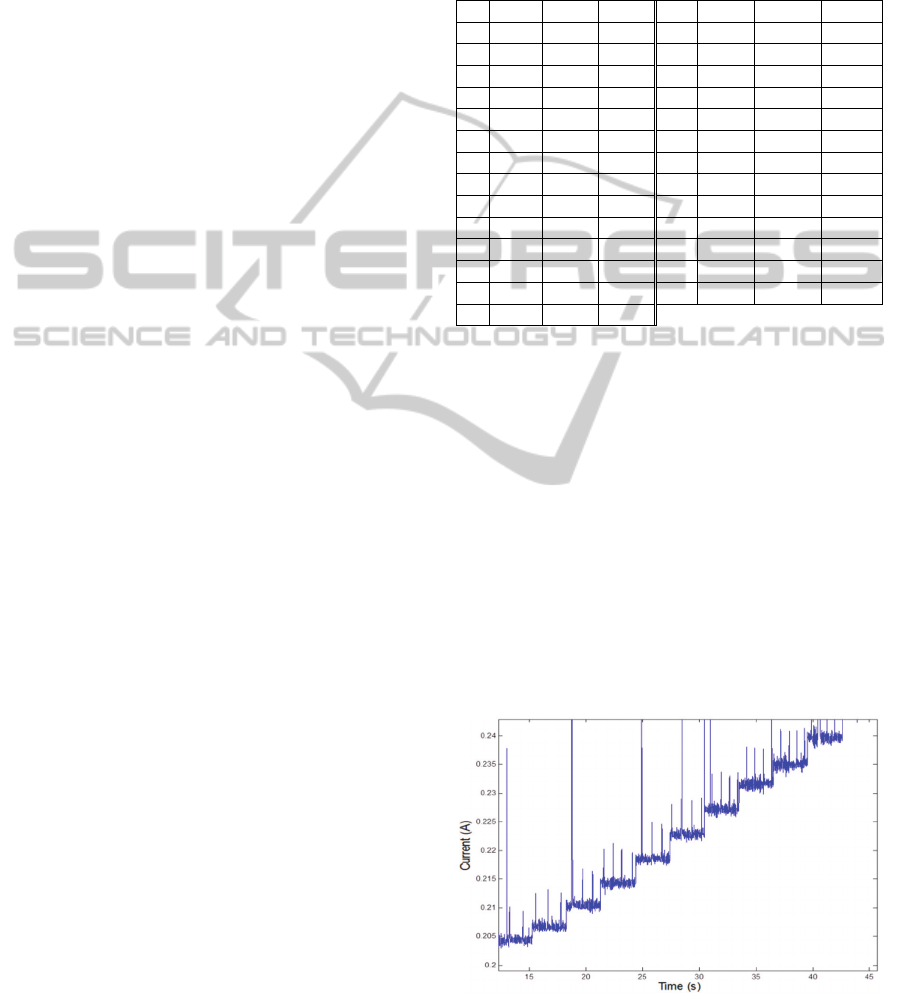
The repetition of the capture experiment for the
same video sequence indicates that there is a certain
basis of (average) consumption for each OPP, more
or less constant for all repetitions, plus a number of
big consumption spikes that appear in different
moments in each repetition. For this reason, those
spikes are not considered to be due to the video task
executed in the CPU but to other “unknown” sinks
in the board. Moreover, by adjusting suitably the
zoom in the graphs, it can be observed, apart from
the biggest “random” consumption spikes, a second
level of pseudo-periodic consumption peaks, whose
period decreases as the OPP frequency increases.
These can be due to accesses to the SD card to get
the video file data packets but not to decoding
activities. Hence, these current peaks should not be
taken into account to model the plant, given that
neither the on-going power estimation procedure
will reflect them. Figure 2 shows these details.
Table 1: OPP data.
No. MHz
a
V
b
A
c
No. MHz
a
V
b
A
c
1 125 0.978 0.186 15 430 1.156 0.245
2 200 0.991 0.197 16 500 1.168 0.259
3 210 1.003 0.199 17 510 1.181 0.263
4 220 1.018 0.201 18 520 1.193 0.266
5 240 1.031 0.205 19 530 1.206 0.270
6 250 1.043 0.207 20 540 1.218 0.274
7 270 1.056 0.211 21 550 1.230 0.278
8 290 1.068 0.215 22 560 1.243 0.282
9 310 1.081 0.219 23 570 1.256 0.288
10 330 1.093 0.224 24 580 1.280 0.290
11 350 1.106 0.228 25 590 1.293 0.297
12 370 1.118 0.233 26 600 1.306 0.301
13 390 1.131 0.236 27 720 1.306 0.327
14 410 1.143 0.241
a
Frequency (MHz);
b
Voltage (V);
c
Average consumption (A)
If the zoom is focused on how the consumption
changes from one OPP to another, the dynamics of
this change can be analyzed. From this analysis, a
mathematical model of the system plant can be
obtained. Thus, for example, starting with a simple
linear first-order Laplace transfer function,
G(s)=1/(2.75·10
-3
s+1) can be obtained (Ogata,
2010), which relates the current consumption with
input OPP average current level. Figure 3 shows the
comparison between the time response of this model
and the actual consumption for an input step from
OPP26 to OPP27 levels. The time response of G(s)
has been compared also with the rest of steps of the
OPP sequence described above and its validity has
been verified.
Figure 2: Detail of the real board consumption profile for
increasing OPPs.
PECCS2015-5thInternationalConferenceonPervasiveandEmbeddedComputingandCommunicationSystems
366
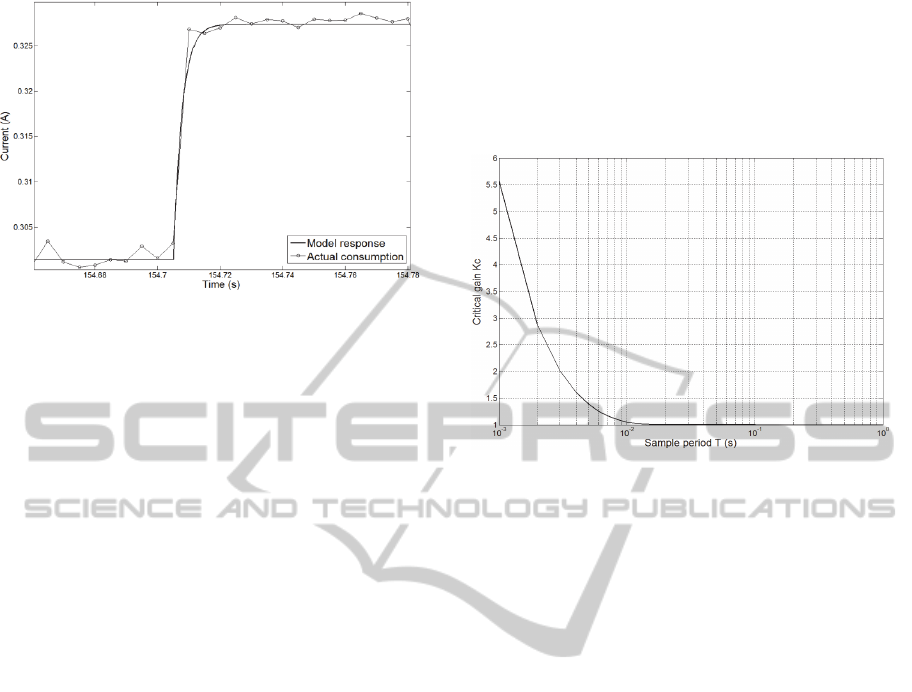
Figure 3: Actual consumption and model response for
OPP26 to OPP27 step.
The proposed model G(s) is a continuous one,
which has to be discretized depending on the action
period T to be considered. If a digital-to-analog
converter (zero-order hold) + continuous process +
analog-to-digital converter (sample & hold) scheme
model is considered for the discretization, a Z
transfer function can be derived from the continuous
model: G(z)=(1-e
pT
)/(z-e
pT
) (Phillips and Parr,
2010), where p is the pole of G(s), i.e. p = –363.63.
5 ANALYSIS AND DESIGN OF
THE CLOSED-LOOP SYSTEM
Once a mathematical model of the plant is obtained,
different analysis techniques can be applied to
foresee the system behavior. A first approach is
addressed with a linear model, which will be
completed later with more realistic (nonlinear)
characteristics.
5.1 Linear Model
Thinking on implementing a closed-loop automatic
power regulation system, one of the parameters to be
fixed is the action period (sample period T of G(z)).
Apart from other technological issues, the stability
of the closed-loop system is one of the
characteristics that must be ensured. As a first
approach, the simplest controller that can be used in
closed loop is a proportional (P) one (Phillips &
Parr, 2010). If we call K the gain of this controller,
the transfer function of the closed-loop system is
M(z)=K(1-e
pT
)/(z-e
pT
+K(1-e
pT
)). Therefore, the
critical gain which leads the system to instability is
K
c
=(1+e
pT
)/(1-e
pT
). If K
c
is represented versus the
sample period, from 1ms to 1s, the graph shown in
Figure 4 is obtained. From that figure it can be
realized that in order to have K
c
values higher than
1, T must be lower than 10ms, which can be a too
low value in terms of system overhead. It is worth
noting that this overhead will come not only from
the execution time of the control algorithm itself but
also from the OPP switching time.
Figure 4: Critical gain of closed-loop system vs sample
period.
Hence, a realistic P controller would have a limit
of 1 for its gain. With this upper bound, the lower
bound for the closed-loop system error in steady
state is min(e
ss
)=100/(1+max(K
c
))=50% (Ogata,
2010), which is too high. In order to avoid this
limitation and still keeping a classic linear
controller, an integral action (I) should be added to
it.
As a first and simple approach to the integral
action, one can choose between a forward and a
backward rectangular rule (FRR and BRR,
respectively) (Franklin and Powell, 1997). Their
corresponding Z transfer functions differ only on a
zero in z=0 which appears in the second case. Given
that for overhead reasons a realistic sample period
cannot be very short, the pole of G(z) will be close
to 0. For example, for a sample time T of 100ms the
pole of G(z) is z=e
pT
=1.6·10
-16
. Therefore, the
practical zero-pole cancellation in a series of a BRR
I and G(z) will enable shorter settling times than
with a FRR I when closing the control loop because
the system dominant pole can be closer to z=0. This
can be deduced from the Z-plane root loci shown in
Figure 5. In the FRR case, the modulus of the
system dominant pole is always greater than or equal
to 0.5, whereas in the BRR case the system
dominant pole can reach the minimum value of 0
thus enabling settling times shorter than the sample
period.
Modeling,AnalysisandDesignofaClosed-loopPowerRegulationSystemforMultimediaEmbeddedDevices
367
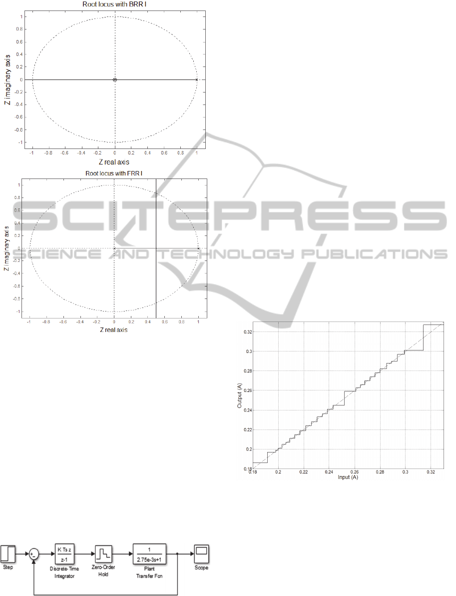
Figure 5: System root locus with BRR (up) and FRR
(down) integrators.
Thus, considering the BRR option, the closed-
loop pole of the system for a long enough sample
period is p
CL
=1-KT, being again K the controller
gain. Let us consider a sample period T of 100ms,
which seems to be a good trade-off value for
keeping reasonable relative overhead, immunity to
jitter effects and frequency of control actions. For
this period, the critical gain which leads the system
to instability (p
CL
=-1) is K
c
=20, whereas the gain for
the shortest settling time (p
CL
=0) is K=10. This is the
gain used for the I controller in the Simulink closed-
loop linear system model of Figure 6, characterized
by null steady-state error and the same settling time
as the plant.
Figure 6: Block diagram of the linear closed-loop control
system.
5.2 Adding Nonlinearities to the
System Model
The initial linear model must be enhanced with more
real system details. For example, perhaps the
clearest nonlinearity of the system is that the
interface to the plant only admits 27 different levels,
i.e. the 27 available OPPs. As mentioned above, this
implies a strong quantization process previous to the
plant, whose steps are even irregular. Hence, the
diagram of Figure 6 must include a block, previous
to the plant, implementing this quantization, which
can even overcome the zero-order hold functionality
and substitute it (see Figure 8). The quantization also
includes implicitly the nonlinear effect of saturation
beyond the limits of the extreme OPPs. From the
OPP average consumption values included in Table
1, the transfer function of this quantization block is
graphically represented with the stepped line of
Figure 7 in 27 irregular steps. The diagonal line of
that figure is a reference to identify how the input
breakpoints should be fixed in the middle of the step
values in order to limit the maximum quantization
error to ±step/2. This is a feature to be added to the
final implementation because our default cpufreq
interface offers both ceil and floor functionality but
not rounding to the nearest valid OPP value.
Figure 7: Transfer function of the discrete OPP
quantization effect.
One of the main advantages of closed-loop
systems is their capability to react to disturbances on
the controlled output. Therefore, the system model
should be completed with a disturbance input, like
shown in Figure 8, in order to analyze its influence.
The disturbance input would simulate the effect of a
consumption variation when the system is following
the set point in steady state, due, for example, to a
variation in the processor load.
PECCS2015-5thInternationalConferenceonPervasiveandEmbeddedComputingandCommunicationSystems
368
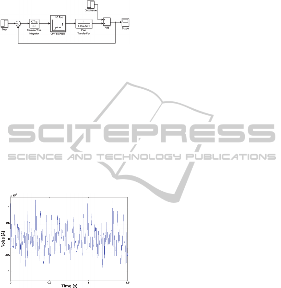
Figure 8: Diagram of the nonlinear closed-loop system
with disturbance input.
Another non-ideal feature that can be added to
the model is what we can call noise in the
consumption signal. I.e. the last column of Table 1
represents average values of current consumption for
each OPP but the actual values do fluctuate around
those averages, as can be distinguished in Figure 3.
If, as explained above, the consumption peaks not
directly due to the video decoding task are omitted
(see Figure 2), then the resulting consumption signal
can be modeled in each OPP as a constant (its
corresponding average value) plus a random-like
“noise” of about 2mA peak to peak and zero mean.
Figure 9 shows an example of this noise. The
disturbance input of the diagram of Figure 8 can be
used to inject a noise like that of Figure 9 into the
system output (consumption) in order to analyze
how it influences the control system.
Figure 9: Simulated noise to be added to the consumption
signal.
6 RESULTS
The Simulink system model of Figure 8 has been
tested in simulation for a number of set points and
disturbances, mainly step shaped. It is worth noting
that a step-shaped input would simulate a constant
current desired for the system consumption (set
point) or modifying the system consumption
(disturbance). In turn, the set-point level might
depend on a number of factors, ranging from system
load to battery state of charge. As a summary, Figure
10 shows the system time response for a set-point
step from OPP1 level to OPP15 level in t=0 and a
disturbance step (undesirable and unexpected
increase of consumption) of a 40% of the input step
in t=0.45s. In that figure it can be seen how, first, the
settling time is shorter than the sample period
(T=100ms) after the initial input step, and second,
the I controller assures a null error in steady state
given that the full target current level is reached after
the settling time (see its corresponding value in
Table 1). Afterwards, with the system consumption
stable at OPP15 level, a sudden consumption
increase arises at t=0.45s and this higher
consumption keeps until the next sample time at
t=0.5s. At that moment, the integral controller
detects the anomaly and corrects it immediately by
decreasing its output to the plant (i.e. by setting a
lower OPP). However, since the disturbance value
probably will imply that there is not any OPP which
cancels exactly its effect, i.e. none OPP applied to
the plant reaches a consumption equal to the target,
the I controller makes the response oscillate.
Something similar would happen also if the set point
did not match any of the OPP levels defined in Table
1, even in the absence of disturbance. The oscillation
in the system current consumption can be seen, on
one hand, as an undesirable behavior of the system,
given that the set point is not oscillating, or, on the
other hand, as the only way the control system can
satisfy the set-point requirement, in average. In fact,
the system is acting as a kind of pulse-width
modulator (PWM), switching between two adjacent
OPPs.
If the disturbance input of Figure 8 is used to
inject the characteristic noise of the system
consumption (see Figure 9) and we let enough
response time, the system output for an example set
point equivalent to OPP3 level is the one shown in
Figure 11. In that figure it can be seen how the
system reaches a current consumption with the
average value of OPP3 (see Table 1), as desired, but
some glitches appear occasionally. What happens is
that, although the average value of the noise is zero,
the sampling process inherent in the control system
may lead to a biased error sequence. This implies
that the integrator output increases or decreases
gradually until it reaches an OPP breakpoint
threshold, thus generating the undesirable glitches of
Figure 11. This can be better understood by
observing Figure 12, which shows the output of the I
controller during the same time interval as in Figure
11. Besides, Figure 12 includes also the two OPP
Modeling,AnalysisandDesignofaClosed-loopPowerRegulationSystemforMultimediaEmbeddedDevices
369
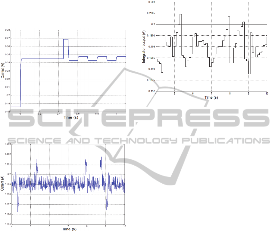
breakpoint levels adjacent to the OPP3 value as a
couple of horizontal lines at 198mA and 200mA,
respectively. The glitches in Figure 11 appear when
the integrator output crosses the breakpoint lines in
Figure 12, which triggers an OPP change.
Figure 10: Closed-loop time response for an OPP1 to
OPP15 input step and disturbance of 40% at t=0.45s.
Figure 11: Closed-loop response for OPP3 level target and
noise disturbance.
The example illustrated in Figure 11 and Figure
12 has been based on an OPP3 target value, the one
closest to its neighbours, as it can be realized from
Table 1. This implies that the glitches in the
consumption will be the lowest but the most
frequent ones, because the integrator output reaches
the breakpoints in less time. In the worst general
case, the highest glitch would have the amplitude of
the highest OPP step, which can be easily identified
in Figure 7 to be between OPP26 and OPP27 with a
value of 26mA from Table 1 data. Anyway, the
glitch width is only one sample period. This issue is
one of the disadvantages of the I controller which
have to be treated, but we will wait to have
consumption estimation data available, in order to
compare its associated noise with that of the actual
consumption used in this paper.
Figure 12: Integrator output for OPP3 level target and
noise disturbance.
7 CONCLUSION AND FUTURE
WORK
A mathematical model of the power consumption
process of a video decoding application running in a
commercial embedded development platform has
been obtained from measured data. Then, classic
analysis and design techniques have been applied to
get a suitable controller able to keep track of the
power consumption in closed loop. Prior to the
availability of real-time power estimation data for
implementing the target system, simulation results
have validated the controller in the presence of
consumption variations. I.e., the control system is
stable and able to make the decoder consumption
follow the set point with a null average steady-state
error regardless the existence of consumption noise
or disturbance. This paves the way for optimizing
the power consumption of multimedia hand-held
devices by applying closed-loop techniques.
From now on, a suitable power estimator has to
be achieved for the video decoder such that its
estimations are as close as possible to the real
consumption. The effects of the possible differences
between estimation and consumption on the control
system have to be analyzed prior to implement the
target system with real-time estimation feedback.
Once the target system is implemented, its response
has to be contrasted with previous simulation results.
This will open the door to further improvements
such as the refinement of the I controller or the test
of different (advanced) controllers. Moreover, the
subsequent power savings will come from the
PECCS2015-5thInternationalConferenceonPervasiveandEmbeddedComputingandCommunicationSystems
370

suitable programming of the set point, which will be
followed by the decoder consumption by means of
the closed-loop control system. The set point will be
programmed to achieve different objectives
involving battery life time, performance or QoE
parameters among others, and the corresponding
power savings will be compared to other existing
solutions in order to evaluate the efficiency of our
proposal. Other further work can lead to more
complex scenarios in which, for example, the
hardware offers more than one CPU, like in
OMAP4-based platforms (TI-Omap4460, n.d.), and
the software is partitioned among different
processing cores. Then the closed-loop control of
power consumption in several CPUs or coprocessors
will be worth researching.
REFERENCES
Agilent 2009, Agilent 14565B Software and 66319B/D
and 66321B/D Mobile Communications DC Sources,
Available from: <http://cp.literature.agilent.com/
litweb/pdf/5990-3503EN.pdf>. [2014.11.26].
Ahmadian, A. S., Hosseingholi, M. and Ejlali, A., 2010. A
control-theoretic energy management for fault-tolerant
hard real-time systems. IEEE International
Conference on Computer Design (ICCD).
Alimonda, A., Carta, S., Acquaviva, A., Pisano, A. and
Benini, L., 2009. A feedback-based approach to DVFS
in data-flow applications. IEEE Transactions on
Computer-Aided Design of Integrated Circuits and
Systems, vol. 28, no. 11, pp. 1691-1704.
Bang, S. Y., Bang, K., Yoon, S. and Chung, E. Y., 2009.
Run-time adaptive workload estimation for dynamic
voltage scaling. IEEE Transactions on Computer-
Aided Design of Integrated Circuits and Systems, vol
28, no. 9, pp. 1334-1347.
Barbalace, A. and Ravindran, B., 2012. Quantitative
evaluation of single and multicore real time DVFS
schedulers in Linux. Technical report available from:
<http://chronoslinux.org/papers/rtdvfs_emb_tech.pdf>.
[2014.12.26]
Beaglboard, n.d. Available from: <http://beagleboard.org/
beagleboard>. [2014.11.26].
Choi, K., Soma, R. and Pedram, M., 2005. Fine-grained
dynamic voltage and frequency scaling for precise
energy and performance trade-off based on the ratio of
off-chip access to on-chip computation times. IEEE
Transactions on Computer-Aided Design of Integrated
Circuits and Systems, vol. 24, no. 1, pp. 18-28.
Franklin, G. F. and Powell, J. D., 1997. Digital Control of
Dynamic Systems. Addison Wesley, 3rd edition.
Gu, Y. and Chakraborty, S., 2008 .Control theory-based
DVS for interactive 3D games. Design Automation
Conference (DAC).
Horvath, T., Abdelzaher, T., Skadron, K., and Liu, X.,
2007. Dynamic voltage scaling in multitier web
servers with end-to-end delay control. IEEE
Transactions on Computers, vol.56, no. 4, pp. 444-
458.
ITU-T and ISO/IEC JTC 1 2012. Advanced Video Coding
for Generic Audiovisual Services. ITU-T Rec. H.264
& ISO/IEC 14496-10.
Jejurikar, R. and Gupta, R., 2004. Dynamic voltage
scaling for systemwide energy minimization in real-
time embedded systems. International Symposium on
Low Power Electronics and Design (ISLPED).
Juárez, E., Pescador, F., Lobo, P., Groba, A. and Sanz, C.,
2010. Distortion-energy analysis of an OMAP-based
H.264/SVC decoder. 6th International Mobile
Multimedia Communications Conference
(MobiMedia).
Le, D. and Wang, H., 2010. An effective feedback-driven
approach for energy saving in battery powered
systems. 18th IEEE International Workshop on
Quality of Service (IWQoS).
Lefurgy, C., Wang, X. and Ware, M., 2007. Server-level
power control. 4th International Conference on
Autonomic Computing (ICAC).
Lu, Z., Lach, J., Stan, M. and Skadron, K., 2003. Reducing
multimedia decode power using feedback control.
International Conference on Computer Design
(ICCD).
Lu, Z., Lach, J., Stan, M. and Skadron, K., 2006. Design
and implementation of an energy efficient multimedia
playback system. Asilomar Conference on Signals,
Systems and Computers.
Minerick, R. J., Freeh, V. W. and Kogge, P. M., 2002.
Dynamic power management using feedback.
Workshop on Compilers and Operating Systems for
Low Power.
Ogata, K., 2010. Modern control engineering, Prentice
Hall, 5th edition.
ORC-RVC-MPEG, n.d. Available from:
<https://github.com/orcc/orc-
apps/tree/master/RVC/src/org/sc29/wg11/mpegh/part2
>. [2014.11.26]
Phillips, C. L. and Parr, J. M., 2010. Feedback Control
Systems, Prentice Hall, 5th edition.
Poellabauer, C., Singleton, L. and Schwan, K., 2005.
Feedback-based dynamic voltage and frequency
scaling for memory-bound real-time applications. 11th
IEEE Real Time and Embedded Technology and
Applications Symposium (RTAS).
Ren, R., Juárez, E., Pescador, F. and Sanz, C., 2012. A
stable high-level energy estimation methodology for
battery-powered embedded systems. 16th IEEE
International Symposium on Consumer Electronics
(ISCE).
Ren, R., Wei, J., Juárez, E., Garrido, M., Sanz, C. and
Pescador, F., 2013. A PMC-driven methodology for
energy estimation in RVC-CAL video codec
specifications. Signal Processing: Image
Communication, vol. 28, no. 10, pp. 1303-1314.
Ren, R., Juarez, E., Sanz, C., Raulet, M., and Pescador, F.,
2014. Energy-Aware decoder management: a case
study on RVC-CAL specification based on just-in-
Modeling,AnalysisandDesignofaClosed-loopPowerRegulationSystemforMultimediaEmbeddedDevices
371

time adaptive decoder engine. IEEE Transactions on
Consumer Electronics, vol. 60, no. 3. pp. 499-507.
RVC-CAL-Sequences, n.d. Available from:
<http://sourceforge.net/projects/orcc/files/Sequences>.
[2014.11.26]
Snowdon, D. C., Petters, S. M. and Heiser, G., 2007.
Accurate on-line prediction of processor and memory
energy usage under voltage scaling. 7th International
Conference on Embedded Software (EMSOFT).
Sullivan, G. J., Ohm, J. R., Han, W. J. and Wiegand, T.,
2012. Overview of the High Efficiency Video Coding
(HEVC) Standard. IEEE Transactions on Circuits and
Systems for Video Technology, vol. 22, no. 12, pp.
1649-1668.
TI-Omap3530, n.d. Available from: <http://www.ti.com/
product/omap3530>. [2014.11.26].
TI-Omap4460, n.d. Available from: <http://www.ti.com/
product/omap4460>. [2014.12.26].
Wang, X. and Wang, Y., 2009. Co-Con: coordinated
control of power and application performance for
virtualized server clusters. 17th IEEE International
Workshop on Quality of Service (IWQoS).
Wang, X., Ma, K. and Wang, Y., 2010. Achieving fair or
differentiated cache sharing in power-constrained chip
multiprocessors. 39th International Conference on
Parallel Processing (ICPP).
Wang, Y., Ma, K. and Wang, X., 2009. Temperature-
constrained power control for chip multiprocessors
with online model estimation. 36th International
Symposium on Computer Architecture (ISCA).
Wu, Q., Juang, P., Martonosi, M., Peh, L. S. and Clark, D.
W., 2005. Formal control techniques for power-
performance management. IEEE Micro, vol. 25, no. 5,
pp. 52-62.
Xia, F., Tian, Y. C., Sun, Y. and Dong, J., 2008. Control-
theoretic dynamic voltage scaling for embedded
controllers. IET Computers & Digital Techniques, vol.
2, no. 5, pp. 377-385.
Zhu, Y. and Mueller, F., 2007. Exploiting synchronous
and asynchronous DVS for feedback EDF scheduling
on an embedded platform. ACM Transactions on
Embedded Computing Systems, vol. 7, no. 1, pp. 3:1-
3:26.
PECCS2015-5thInternationalConferenceonPervasiveandEmbeddedComputingandCommunicationSystems
372
