Multi-modal Transportation with Public Transport and Ride-sharing
Multi-modal Transportation using a Path-based Method
Sacha Varone
1
and Kamel Aissat
2
1
University of Applied Sciences and Arts Western Switzerland (HES-SO), HEG Gen
`
eve, Gen
`
eve, Switzerland
2
LORIA, University of Lorraine, Nancy, France
Keywords:
Multi-modal, Public Transportation, Ride-sharing, Real-time, Geographical Maps.
Abstract:
This article describes a multi-modal routing problem, which occurs each time a user wants to travel from a
point A to a point B, using either ride-sharing or public transportation. The main idea is to start from an
itinerary using public transportation, and then substitute part of this itinerary by ride-sharing. We first define a
closeness estimation between the user’s itinerary and available drivers. This allows to select a subset of poten-
tial drivers. We then compute sets of driving quickest paths, and design a substitution process. Finally, among
all admissible solutions, we select the best one based on the earliest arrival time. We provide numerical results
using benchmarks based on geographical maps, public transportation timetabling and simulated requests and
driving paths. Our numerical experiment shows a running time of a few seconds, suitable for a new real-time
transportation application.
1 INTRODUCTION
The growth of the nation and the need to meet mo-
bility, environmental, and energy objectives require
other alternative transportation systems. In fact, pub-
lic transportation systems are insufficient to address
the needs of passengers in terms of flexibility and
cost. One potential solution to meet these require-
ments without expanding service area or increas-
ing service frequency of public transportation, is to
jointly consider ride-sharing services. In this pa-
per, we explain a methodology able to combine in
a same journey from an origin to a destination, pub-
lic transportation and ride-sharing. This mix provides
new aspects of the mobility, which combines fixed
timetabling from public transportation and highly dy-
namic ride-sharing, and might also be an interesting
transportation business.
We consider the following situation: a user, called
a rider, wishes to travel from an origin to a destination
at a given time. His goal is to reach his destination as
quickly as possible, using either public transportation
and walking, or ride-sharing. He might enter the sys-
tem at any time, being considered as a request. Other
users called drivers offer to share all or part(s) of their
drive, even at the price of a (not too long) detour; they
also have origins, destinations and starting times. The
system first find a public transportation path that sat-
isfies the rider’s request, and then tries to sequentially
substitute part of the rider’s public transportation path
with ride-sharing path.
A network, combining public transportation and
driving networks, is modelled as a directed graph
G(V,E), V being the set of nodes and E the set of arcs.
Nodes represent intersections and arcs describe street
segments. A non negative function, called a cost, is
associated with each arc; it determines the driving du-
ration between two nodes. A quickest path, which
is also a shortest path in our network, is a path that
minimizes the sum of its costs. A stop is defined as
the location for which a transit or road node exists.
Stops correspond to bus stops, subway stations, park-
ings, etc. We describe in this paper an algorithmic
approach to the real-time multi-modal earliest-arrival
problem (EAP) in urban network, using ride-sharing
and public transportation.
The paper is organized as follows: Section 2
presents a brief literature review. Section 3 explains
the algorithmic process and its complexity, each step
being illustrated with an example. Finally, Section
4 presents insight about its efficiency and gives con-
cluding remarks.
479
Varone S. and Aissat K..
Multi-modal Transportation with Public Transport and Ride-sharing - Multi-modal Transportation using a Path-based Method.
DOI: 10.5220/0005366204790486
In Proceedings of the 17th International Conference on Enterprise Information Systems (ICEIS-2015), pages 479-486
ISBN: 978-989-758-096-3
Copyright
c
 2015 SCITEPRESS (Science and Technology Publications, Lda.)

2 BACKGROUND
The growth of recent advancements in technology is
progressing day by day. This leads to increase in
transportation facilities. Specifically, the use of GPS-
enabled smartphone has increased the possibilities to
match riders and drivers, which is nowadays done in
quasi real-time (see for example (Chan and Shaheen,
2012)). The concept of ride-sharing is close to the dy-
namic Dial A Ride Problem, in which rides’ requests
have to be fulfilled in real-time with one (or some-
times several) vehicle(s), starting from a depot. The
latter problem is a special case of pick-up and deliv-
ery problems, in which requests have to be fulfilled
for users instead of goods. The main difference is that
in ride-sharing, there is no depot, but a list of Origin-
Destination drives which might change to pick-up and
drop-off some riders. A recent survey of the pick-up
and delivery problem can be found in (Berbeglia et al.,
2010), and recent survey for dynamic ride-sharing
problems has been done in (Agatz et al., 2012). The
background of dynamic ride-sharing is the ability to
compute shortest paths. This problem has been well
studied by researchers and very efficient algorithms
allow to solve this problem on continental size in-
stances within a few milliseconds. Recent advances
in route planning algorithms can be found in (Bast
et al., 2014), which updates the survey of (Delling
et al., 2009).
Multi-modal itinerary computation for ride-
sharing does not only include shortest paths calcula-
tion, but also multi-criteria paths, transition or waiting
times, etc. which is usually not taken into account in
shortest paths on pure road networks. The authors in
(Ambrosino and Sciomachen, 2014) use for example
an objective with several features and consequently
focus almost exclusively on the modal change node.
They provide a two-step algorithm for the computa-
tion of multi-modal routes. In (Liu et al., 2014), an
exact algorithm is given for a ride-sharing problem
with arrivals and departures time-windows. Multi-
criteria search has been proposed by (Herbawi and
Weber, 2012) using genetic algorithm or by comput-
ing the Pareto set in (Delling et al., 2013).
Public transportation problems have received a lot
of attention, solving earliest-arrival problems (EAP)
knowing departure time and station, arrival station
and timetable information. A review of this topic can
be found in (M
¨
uller-Hannemann et al., 2007; Pyrga
et al., 2008). The two main multi-modal networks are
described, namely, the time-expanded graph and the
time-dependent graph. Our approach uses the time-
dependent graph, since does not explode the number
of nodes. Timetabling information and EAP solving
is nowadays often available on-line, either via a web
browser or via requests to a restful server. In some
cases, timetables information might not be accurate
and approximations based on probability distribution
might be applied, as done in (Murueta et al., 2014).
Our approach considers that such a service is avail-
able.
Real-time journey computation for ride-sharing
opportunities faces the commuting point problem: the
detection of the pick-up and drop-off locations are
part of the problem. This problem is defined in (Bit-
Monnot et al., 2013) define as the 2 synchronization
points shortest path problem (2SPSPP). More pre-
cisely, for a given driver and a rider, authors propose
an optimal method to find the pick-up and drop-off
locations in O(m·n
2
), where n is the number of nodes
and m is the number of edges in the graph. Their ob-
jective function minimizes the cumulated travel time
of driver and rider. The time complexity of this ap-
proach does not allow its use in real-time ride-sharing,
and their model does not take into account the driver’s
detour time constraint, i.e. the total time of the detour
should be less than a given threshold specified for the
driver.
Our approach starts with the finding of a short-
est path using public transportation. As the differ-
ent transit stops are given by the path so far discov-
ered, pick-up and drop-off are only allowed around
those stops in order to reduce the search space. More-
over, we also consider the best offer selection prob-
lem, i.e. for a given rider, we select the best driver that
improves the rider’s itinerary by setting the different
transit stops as potential pick-up and drop-off loca-
tions, under driver’s detour time and driver’s waiting
time constraints.
3 APPROACH: SUB-PATH
SUBSTITUTION
We define now the problem to be solved: a rider u
wishes to go from an origin point O
u
to a destina-
tion point D
u
. He might use either public transporta-
tion, ride-sharing or a combination of both. All public
transportation timetabling are assumed to be known
or at least accessible easily. In Switzerland, one might
use the Swiss public transport API (Application Pro-
gramming Interface)
1
; in France, a similar service is
available
2
. The origin-destination (OD) couple of po-
tential ride-sharing drivers are also detected and lo-
cated in real-time.
1
http://transport.opendata.ch
2
http://www.navitia.io
ICEIS2015-17thInternationalConferenceonEnterpriseInformationSystems
480

Throughout this section, together with the de-
scribed algorithmic process, we present an illustra-
tive example in order to better understand the differ-
ent steps that constitute our approach. The example
represents the following situation: a user u requests to
travel from an origin O
u
to a destination D
u
, starting at
time t
u
= 9:00. Public transportation allows him to go
from a point x
2
to another point x
nbs
, close to respec-
tively points O
u
and D
u
, via points x
2
,x
3
,..., x
nbs−1
.
In order to simplify the understanding, our illustrative
example supposes that the origin O
u
is already a bus
stop, hence O
u
= x
1
. For simplicity again, only one
driver k is considered (see Figure 3-9).
The public transportation path is noted as P =
O
u
,x
2
,..., x
nbs
,D
u
, its successive points are called
“stops”. Note that “nbs” stands for number of stops.
Let’s call OD the set of origin-destination couple
of users. An element O
k
D
k
∈ OD is characterized by
its origin O
k
, its destination D
k
and its starting time t
k
0
for user k.
Notation :
s e driving quickest path between s and e.
δ(s,e) duration of a quickest path between s
and e.
d(s, e) distance as the crow flies between s
and e.
ˆ
δ(s,e) estimated smallest duration from s to e
ˆ
δ(s,e) =
d(s,e)
v
max
, where v
max
is the
maximal speed.
λ
k
detour coefficient of driver k, λ
k
≥ 1.
τ(x)
ab
time required for moving from modality
a to b at x.
t
u
a
(x,m) arrival time at x using the m transport
modality for user u.
t
u
d
(x,m) departure time at x using the m transport
modality for user u.
w
k
max
maximum waiting time for driver k
at pick-up point.
LP
↓
k
forward search space from O
k
.
LP
↑
k
backward search space from D
k
.
We will further note as p the public transportation
modality, and as c the car modality.
3.1 Initial Request Processing
As a ride request O
u
D
u
arrives in the system at time
t
0
, a shortest path using public transportation is pro-
cessed, as well as possible driving substitution sub-
paths along the public transportation path. This is the
purpose of Algorithm 1.
Step 1 gives the path P using public transportation,
with its arrival time and departure time on each of its
commute node between position O
u
and destination
Algorithm 1: Initial request processing.
Require: Demand O
u
D
u
,t
0
Ensure: Path P
Driving quickest sub-paths
PDrive
1: Find path P = O
u
,x
1
,..., x
nbs
,D
u
using public
transportation API, starting in O
u
at time t
0
, with
its associated arrival times t
u
a
(x, p) and departure
times t
u
d
(x, p), x ∈ P.
2: Compute driving quickest paths along P, with its
associated arrival times t
u
a
(x,c), x ∈P.
3: Set PDrive :=
/
0
4: for all x,y ∈ P, x before y do
5: if t
u
a
(x, p) + τ(x)
pc
+ δ(x,y) ≤t
u
a
(y, p) then
6: PDrive := PDrive ∪{(x, y)}
7: end if
8: end for
9: LDriver =
/
0
D
u
. Step 2 computes possible driving substitution
paths along P. Only those whose arrival time at the
drop-off stop is less than the arrival time using pub-
lic transportation are kept. The time at the poten-
tial pick-up stop plus the transshipment time plus the
ride-sharing time until stop y, is compare to the ar-
rival time at y without ride-sharing. If the gain in time
for the user is not positive, then the considered ride-
sharing (x,y) is not admissible. The admissible ride-
sharing set is defined by PDrive. Step 9 initializes
a list LDriver of potential drivers associated with the
current rider u.
Figure 1 illustrates an instance where a rider u
travels at starting time t
u
= 9:00 from his origin O
u
,
which is also the first stop x
1
, to his destination D
u
.
Figure 1 represents the situation after step 1 of Algo-
rithm 1. For each stop x
i
∈ P, we associate a time
window [t
u
a
(x
i
, p), t
u
d
(x
i
, p)] that represents the arrival
time at the stop x
i
and the departure times from stop
x
i
, respectively. The path found by the API is com-
posed of three different modes. The rider waits at his
origin 3 minutes before boarding the bus at 9:03, then
he is dropped off at stop x
2
, walks from stop x
2
to stop
x
3
during 5 minutes, and finally waits 5 more minutes
before taking the train to reach his final destination
D
u
(see Figure 1).
O
u
D
u
x
2
x
3
5
Bus
20
Walking
26
Train
[9,9 : 03]
[9 : 23,9 : 23] [9 : 28,9 : 33] [9 : 59,9 : 59]
Figure 1: Path P using public transportation.
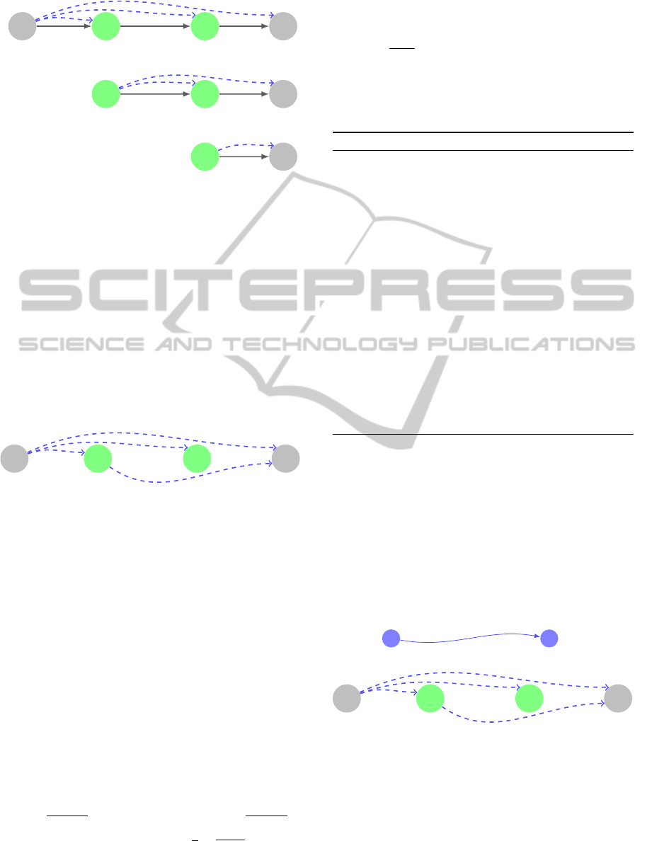
Figure 2 represents step 2 of Algorithm 1, where
all potential driving substitution sub-paths are com-
puted.
Multi-modalTransportationwithPublicTransportandRide-sharing-Multi-modalTransportationusingaPath-based
Method
481

O
u
D
u
x
2
x
3
520 26
16
36
15
[9,9 : 03]
[9 : 23,9 : 23] [9 : 28,9 : 33] [9 : 59,9 : 59]
D
u
x
2
x
3
5 26
6
30
[9 : 23,9 : 23] [9 : 28,9 : 33] [9 : 59,9 : 59]
D
u
x
3
26
31
[9 : 28,9 : 33] [9 : 59,9 : 59]
Figure 2: Quickest driving paths for every pair (x
i
,x
j
) such
that stop x
j
is situated after stop x
i
are shown as dashed blue
line.
In Figure 3 are shown the admissible potential
substitution sub-paths, returned by Algorithm 1. The
ride-sharing path (x
2
,x
3
) would results in an arrival
time at x
3
later than that one if public transporta-
tion is use, since it requires 6 minutes from x
2
to
x
3
, rather then 5 minutes. A similar situation occurs
for the ride-sharing path (x
3
,D
u
): 31 minutes of ride-
sharing compared to 26 minutes by public transporta-
tion. Therefore both sub-paths (x
2
,x
3
) and (x
3
,D
u
)
are canceled.
O
u
D
u
x
2
x
3
16
36
30
15
Figure 3: Admissible driving substitution arcs.
3.2 Closeness Estimation
We define an estimate on how close is a substitution
driving path OD to a public transportation sub-path of
P. This estimated distance is defined as the minimal
sum of the estimated distance from a vertex in OD
to a vertex in P, and backward from P to OD. Four
different points are used, so that only non-trivial sub-
stitution are allowed (i.e. no substitution of a single
vertex). For that purpose, we estimate the distance
between two points given by their latitude/longitude
with the Haversine formula.
This formula uses a spherical model to estimate
the distance between two points x = (λ
1
,θ
1
) and y =
(λ
2
,θ
2
) on the earth surface.
a = sin(
θ
2
−θ
1
2
)
2
+cos(θ
1
)∗cos(θ
2
)∗sin(
λ
2
−λ
1
2
)
2
d(x, y) = R ∗2 ∗atan2(
√
a,
√
1 −a)
where λ
i
,i = 1,2 are the latitudes, θ
i
,i = 1,2 are the
longitudes, R ≈6371 [km] is the earth’s radius. Thus,
the estimated smallest duration from x to y is noted by
ˆ
δ(x,y) =
d(x,y)
v
max
, such that v
max
is the maximal speed
of a car in concerned area. This is a solution to the so
called great-circle distance between two points prob-
lem (sometimes also called “orthodromic distance”
problem).
Algorithm 2: Closeness substitution sub-path for driver k.
Require: Path P, λ
k
, O
k
D
k
of a driver, PDrive,
LDriver
Ensure: Potential pick-up locations LP
↓
k
Potential drop-off locations LP
↑
k
Update LDriver.
1: LP
↓
k
:=
/
0, LP
↑
k
:=
/
0
2: for each (x,y) ∈ PDrive do
3: Estimate
ˆ
δ(O
k
,x) from O
k
to x
4: Estimate
ˆ
δ(y, D
k
) from y to D
k
5: if
ˆ
δ(O
k
,x) + δ(x,y) +
ˆ
δ(y, D
k
) ≤ λ
k
δ(O
k
,D
k
)
then
6: Update LP
↓
k
:= LP
↓
k
∪{x}
7: Update LP
↑
k
:= LP
↑
k
∪{y}
8: Update LDriver := LDriver ∪{k}
9: end if
10: end for
Algorithm 2 restricts the list of potential drivers to
those whose OD is close enough to P, and whose de-
tour time is less than a threshold value. Step 5 checks
if the driver’s time from his origin to destination in-
cluding the detour via x and y is less than its maximal
detour bound.
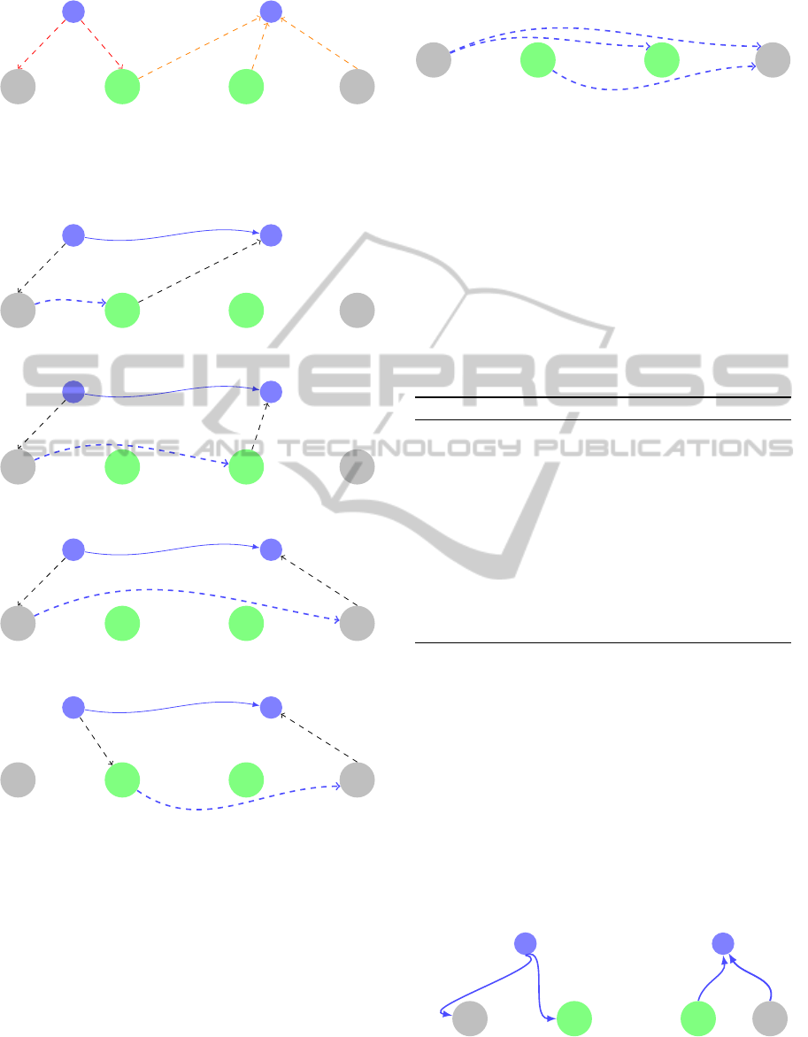
Figure 4 shows the situation at the beginning of
Algorithm 2. In the next steps describing Algorithm
2, driver’s detour should not exceed more than 20%
of his initial trip duration (i.e. λ
k
= 1.2).
O
u
D
u
x
2
x
3
D
k
O
k
t
0
= 9:02
16
36
30
15
47
Figure 4: Driver k drives from O
k
to D
k
, starting at time
9:02. Nodes in path P with potential ride-sharing sub-paths
are shown in dashed blue lines.
Figure 5 shows the results of the estimation based
on the Haversine formula.
Figure 6 shows each potential substitution sub-
path, starting from the driver’s origin and ending to
ICEIS2015-17thInternationalConferenceonEnterpriseInformationSystems
482

O
u
D
u
x
2
x
3
22
O
k
D
k
1316 26
4
Figure 5: Estimation of the duration to each potential pick-
up nodes, and from each potential drop-off nodes, for driver
k, using the Haversine formula. Each geographical position
are supposed to be known.
O
u
D
u
x
2
x
3
O
k
D
k
15
47
(a)
16
26
O
u
D
u
x
2
x
3
O
k
D
k
16
47
(b)
16
22
O
u
D
u
x
2
x
3
O
k
D
k
36
47
(c)
16
4
O
u
D
u
x
2
x
3
O
k
D
k
30
47
(d)
4
13
Figure 6: All potential substitution sub-paths are evaluated
against the detour constraint.
the driver’s destination. The numbers on the segments
represent the estimated duration, whereas the num-
bers along the blue arcs represent the true duration, as
computed in Algorithm 1.
Figure 7 shows the result of Algorithm 2, where
arc (O
u
,x
2
) has been removed since ride-sharing on
this path would implies to drive during 16+15+26 =
57 minutes, exceeding the detour limit of 1.2 ×47 =
56.4 minutes. Then, we remove the potential driving
substitution arc (O
u
,x
2
) because the lower bound of
O
u
D
u
x
2
x
3
16
36
30
Figure 7: Only potential substitution sub-paths that do not
violate the detour constraint are kept.
driver’s detour duration is not satisfied. This allows
to restrict the list of potential pick-up and drop-off
locations
3.3 Shortest Paths Computation
Once a driver k is classified as a potential driver in
LDriver, we compute with Algorithm 3 a set of short-
est paths in order to check the exact constraints of time
detour and waiting time.
Algorithm 3: Paths computation to/from P for driver k.
Require: Demand O
u
D
u
, O
k
D
k
of a driver,
Public transportation database (API)
Potential pick-up locations LP
↓
k
Potential drop-off locations LP
↑
k
.
Ensure: Set of quickest paths to pick-up locations LO
k
Set of quickest paths from drop-off locations LD
k
1: Compute driving quickest paths to LP
↓
k
LO
k
= O
k

x ∈LP
↓
k
\{D
u
}

2: Compute driving quickest paths from LP
↑
k
LD
k
=

y ∈LP
↑
k
\{O
u
}

D
k
Algorithm 3 provides a set of computed shortest
paths. It serves as a basis to substitute part of the P
public transportation path with a ride-sharing modal-
ity. Step 1 constructs shortest driving paths from the
position of the driver to each of the nodes in LP
↓
k
, ex-
cept the last one D
u
. The goal is to find a driving
way to possible commutation points. Step 2 computes
driving paths from nodes in LP
↑
k
, except the first one
O
u
, to the driver’s destination D
k
. Such a path will be
used once a driver has dropped off a rider, and then
have to find his route back to his destination D
k
. (see
Figure 8)
O
u
D
u
x
3
x
2
D
k
O
k
23 616
17
Figure 8: Exact driving paths computation. Only quickest
paths from the origin to admissible pick-up and from ad-
missible drop-off to destination are computed.
Multi-modalTransportationwithPublicTransportandRide-sharing-Multi-modalTransportationusingaPath-based
Method
483

3.4 Substitution Process According to
Time-savings
We only consider feasible substitution sub-paths that
do not increase the arrival time of the rider to his des-
tination. For that purpose we introduce the notion of
reasonable substitution sub-path with the following
definition:
Definition 3.1. (Reasonable Substitution Sub-path)
We say that an arc (x,y) form a reasonable substitu-
tion sub-path for the driver k and the rider u if and
only if the maximal waiting time w
k
max
constraint for
the driver k at a pick-up location (1), the maximum
detour constraint (2) for the driver k, and the latest
arrival time constraint (3) for the rider u are satis-
fied, i.e,
t
u
a
(x, p) + τ(x)
pc
−t
k
a
(x,c) ≤ w
k
max
waiting (1)
δ(O
k
,x) + max

t
u
a
(x, p) + τ(x)
pc
−t
k
a
(x,c),0

+δ(x,y) + δ(y,D
k
) ≤ λ
k
δ(O
k
,D
k
) detour (2)
max

t
k
a
(x,c),t
u
a
(x, p) + τ(x)
pc
}
+δ(x,y) ≤t
u
a
(y, p) arrival (3)
Constraints (1), (2) and (3) take into account
time required for moving from public transportation
modality to ride-sharing modality.
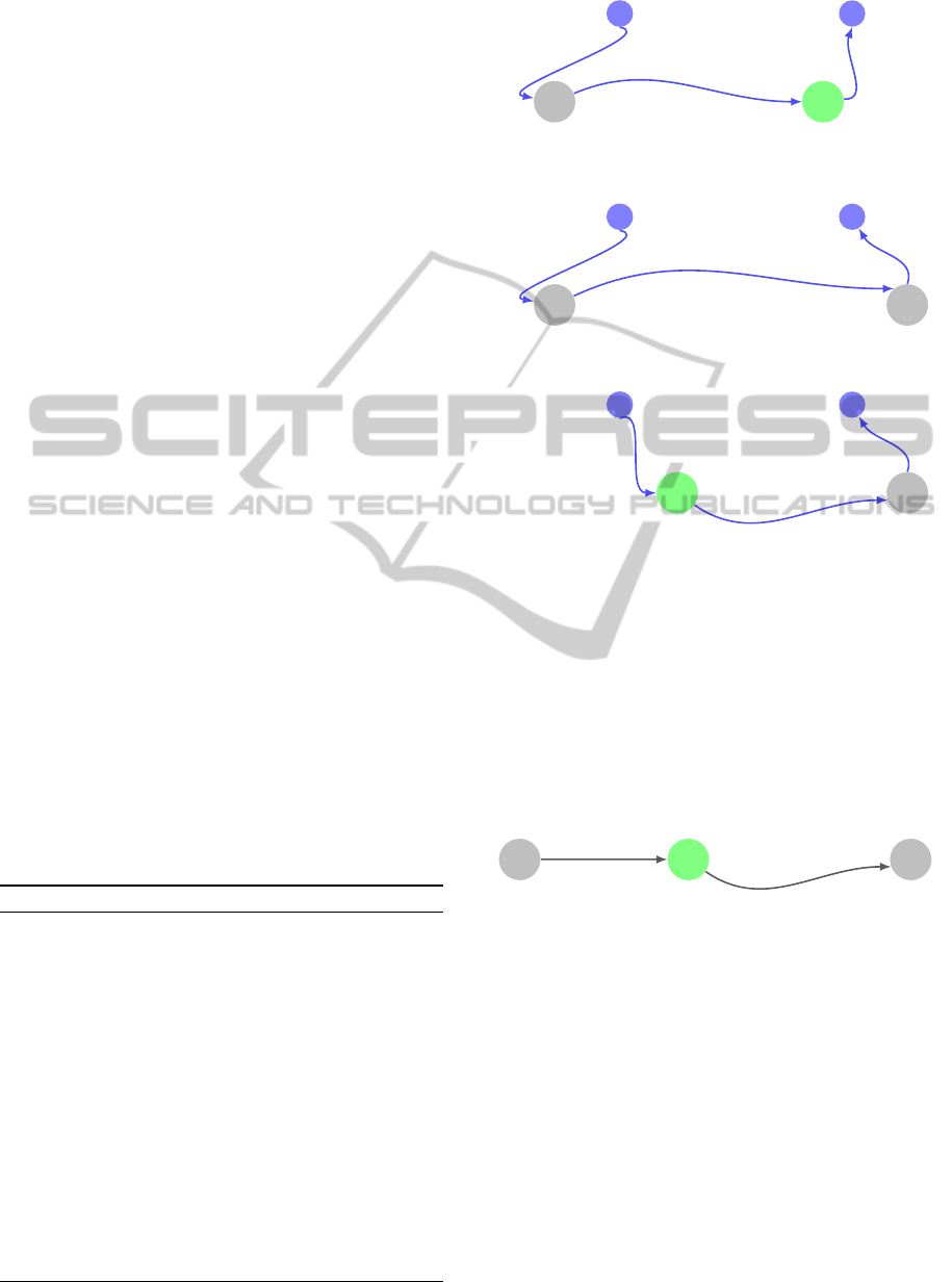
The objective function that defines the best substi-
tution sub-path is based on time-savings: among all
reasonable substitution sub-path, we select the best
substitution sub-path (x,y) that generates for the rider
the most positive time-savings, if he uses ride-sharing
with driver k from the pick-up stop x to the drop-off
stop y rather than public transportation (see Figure 9).
Algorithm 4 defines this process.
Algorithm 4: Best substitution sub-path with driver k.
Require:Demand O
u
D
u
, O
k
D
k
of a driver, A
1
, A
2
, A
3
Ensure: Best substitution sub-path (x
?
,y
?
) or failed
insertion
1: Initialization: σ
?
← 0
2: for each (x, y) in the substitution sub-path set do
3: if (x, y) form a reasonable substitution sub-path
for driver k and rider u then
4: σ = t
u
a
(y, p) −

max{t
k
a
(x,c),t
u
a
(x, p) +
τ(x)
pc
}+ δ(x,y)

5: if σ
?
≤ σ then
6: σ
?
← σ
7: Update the best substitution sub-path
(x
?
,y
?
)
8: end if
9: end if
10: end for
O
u
x
3
9:28 - 9:35 = -0:07 ≤ 0
D
k
O
k
t
k
0
= 9:02
t = 9:19
waiting time before pick-up = 0
(a)
t = 9:35
16
17
23
O
u
D
u
D
k
t = 9:19
waiting time before pick-up = 0
(b)
O
k
t
k
0
= 9:02
9:59-9:55 = 0:04
17
6
t = 9:55
36
D
u
x
2
6
16
D
k
O
k
t
k
0
= 9:02
30
t = 9:53
9:59-9:53 = 0:06
t = 9:18
waiting time before pick-up = 5
(c)
Figure 9: Best substitution sub-path. Ride-sharing (O
u
,x
3
)
increases the earliest arrival time at x
3
; therefore it is can-
celed. Between ride-sharing (O
u
,D
u
) and (x
2
,D
u
), the last
one better improves the arrival time at D
u
; it is therefore the
best substitution sub-path.
Note that from a drop-off location, the rider’s
route have to be recomputed to take into account his
new arrival time. In this example, the drop-off loca-
tion corresponds to the destination of rider. The new
itinerary of the rider is represented in Figure 10.
O
u
D
u
x
2
[9,9 : 03]
[9 : 23,9 : 23]
20
30
Ride-sharing
[9 : 53,9 : 53]
Bus
Figure 10: New itinerary of the rider.
Finally, in order to find the best substitution sub-
path among all drivers, it remains to scan each driver
k in the driver’s list LDrivers and select the driver k
?
that generates the best substitution sub-path (x
?
,y
?
).
This is done by Algorithm 5. It is to be noted that
from y
?
, the rider’s route have to be recomputed in
order to take into account his new arrival time at y
?
.
Therefore, the path P is updated, using y
?
as the new
origin (Step 13). The new starting time t
0
0
is its arrival
time at y
?
(Step 12). The driver’s route is then O
k
?
x
?
y
?
D
k
?
(Step 15). In our example, the new
itinerary of the driver k will become O
k
x
2
D
u
D
k
.
ICEIS2015-17thInternationalConferenceonEnterpriseInformationSystems
484

Algorithm 5: Best substitution sub-path among all drivers.
Require: Demand O
u
D
u
,t
0
Ensure: Best substitution sub-path among all drivers
or failed insertion
1: Initial request processing using Algorithm 1
2: for each driver k ∈ LDriver do
3: Compute the closeness substitution sub-path
for driver k, using Algorithm 2
4: if k ∈LDriver then
5: Compute the paths to/from LP
↓
k
/LP
↑
k
for
driver k, using Algorithm 3
6: Find the best substitution sub-path with
driver k, using Algorithm 4
7: Update the best substitution sub-path
(x
?
,y
?
) with associated driver k
?
8: end if
9: end for
10: Substitution of x to y in P with x
?
y
?
11: if y
?
6= D
u
then
12: t
0
0
= max{t
k
a
(x
?
,c),t
u
a
(x
?
, p) + τ(x
?
)
pc
} +
δ(x
?
,y
?
)
13: Find the path P
0
= y
?
...D
u
using public trans-
portation API, starting at time t
0
0
14: end if
15: Update the driver’s route to O
k
?
x
?
y
?
D
k
?
.
3.5 Complexity
We describe the complexity of the whole process in
a worst case analysis. Algorithm 1 initializes the re-
quest processing in O(D
road
·(|P|−1) + D
API
)-time,
where D
road
(resp. D
API
) is the complexity of the Di-
jkstra algorithm in a road (resp. multi-modal) net-
work. Algorithm 2, which allows to determine the
driver’s admissibility to join the rider’s trip, runs in
O(|PDrive|)-time. Then, in order to check the exact
detour time constraint of the driver, Algorithm 3 al-
lows to compute two sets of shortest paths in the road
network, one from the driver’s origin to stops (LO
k
)
and another from the stops toward the driver’s desti-
nation (LD
k
). Thus, its complexity is in O(2 ·D
road
).
Having the two sets LO
k
and LD
k
as input, Algorithm
4 finds the best substitution sub-path with driver k that
satisfy the maximum driver’s detour time and runs in
O(|PDrive|)-time. Finally, Algorithm 5 uses as sub-
routine the previously described algorithms. We note
that Algorithms 2, 3 and 4 have to be run for each
driver k in the set LDriver. Therefore, the complexity
of the whole process described by Algorithm 5 is in
O

D
road
·(|P|−1)+D
API
+2·|LDriver|·(|PDrive|+
D
road
)

.
In order to reduce the complexity time of our
approach, we focus on the number of stops rather
than the number of drivers. More precisely, instead
of computing for each driver k two Dijkstra algo-
rithms, one from the driver’s origin to stops (LO
k
)
and another from the stops towards the driver’s des-
tination (LD
k
), we simply compute for each poten-
tial pick-up stop one Dijkstra algorithm with back-
ward search from the origins of potential drivers con-
tained in |LDrive| towards the stop. And for each
potential drop-off location, we compute one Dijkstra
algorithm with forward search from each potential
drop-off location towards drivers’ destinations. So,
we compute |P
+
|+ |P
−
| Dijkstra algorithms instead
of 2 ·|LDrive|·|PDrive|, where |P
+
| and |P
−
| are re-
spectively the number of potential pick-up and drop-
off locations. Thus the complexity time is reduced to
O

D
road
·(|P|−1) + D
API
+ 2 ·|LDrive|·|PDrive|+
|P
−
|·D
road
+ |P
+
|·D
road

.
4 NUMERICAL RESULTS AND
CONCLUSION
The methodology to test our approach is based on
simulations, since we are not aware of benchmarks
that fit the problem we solve. We first chose k clus-
ters corresponding to k = 4 cities in Switzerland (Fri-
bourg, Lausanne, Bern, Neuch
ˆ
atel). We then create
L
r
= 10 requests between each pair of clusters, start-
ing randomly between 7:00 and 8:00 AM on a week-
day. For each request, we retrieve public transporta-
tion from available API. We then create L
d
= 5 driv-
ing trips close enough from the stops given by pub-
lic transportation segments, using geographical maps
from OpenStreetMap
3
, as well as routing process
available through the open source tool Osmsharp
4
.
We then apply our algorithms to measure the gain in
terms of arrival time, as well as the running time of
our algorithms.
Our simulation only give some indications about
the efficiency of our approach, which has to be more
deeply investigated by means of real data. First, the
complete process is able to run on a personal com-
puter and only require only a few seconds. Moreover
this slightly depends on geographic density of drivers
around a rider itinerary. One of the reasons for a so
small running time is mainly due to the filtered nature
of Algorithm 2, which considerably reduces the list of
potential drivers. Considering these results, a true ap-
plication is viable through the use of smartphone and
a central server.
Second, there is a significant gain for the rider
3
http://www.openstreetmap.org
4
http://www.osmsharp.com
Multi-modalTransportationwithPublicTransportandRide-sharing-Multi-modalTransportationusingaPath-based
Method
485

in terms of arrival time. Nevertheless the objective
function might miss some features, but can be rede-
fined as a weighted mean of total monetary cost for
the rider, deviation from the origin-destination trip for
the driver, number of transshipment stops, etc. An-
other way to deal with several features might be the
use of a multi-objective function and the computation
of Pareto optimal solutions.
To conclude, the problem described in this pa-
per can be seen as a new multi-modal transportation
design. The originality of our approach is its abil-
ity to also include a ride-sharing modality, along the
more common pedestrian, cycling, private car or pub-
lic transportations modes.
The particular interest of our work is in making
the service of ride-sharing and public transportation
more flexible and efficient. Specifically, in contrast to
the traditional ride-sharing service, our approach al-
lows to reduce the driver’s detour by using intermedi-
ate pick-up and drop-off locations for the rider, and to
increase the savings for both drivers and riders, com-
pared to the traditional ride-sharing service. The ride-
sharing service can be considered as a complement to
transit for public transportation, i.e. the ride-sharing
will improve transportation service in rural areas, dif-
ficult to serve by public transportation only.
This is the main reason that will incite the public
transport agencies to use ride-sharing to complement
their services. Despite the relative importance of inte-
grating ride-sharing into public transport services, as
far as we know, no previous work exists that allows
to deal with this problem in dynamic and real-time
context. One of the reasons could be the difficulty
to define and combine in real-time the two services:
ride-sharing and public transportation.
ACKNOWLEDGEMENTS
This research was partially funded thanks to the swiss
CTI grant 15229-1 PFES-ES received by the first au-
thor.
REFERENCES
Agatz, N. A. H., Erera, A. L., Savelsbergh, M. W. P., and
Wang, X. (2012). Optimization for dynamic ride-
sharing: A review. European Journal of Operational
Research, 223(2):295–303.
Ambrosino, D. and Sciomachen, A. (2014). An algorith-
mic framework for computing shortest routes in urban
multimodal networks with different criteria. Procedia
- Social and Behavioral Sciences, 108(0):139 – 152.
Operational Research for Development, Sustainability
and Local Economies.
Bast, H., Delling, D., Goldberg, A., M
¨
uller-Hannemann,
M., Pajor, T., Sanders, P., Wagner, D., and Werneck,
R. (2014). Route planning in transportation networks.
MSR-TR-2014-4 8, Microsoft Research.
Berbeglia, G., Cordeau, J., and Laporte, G. (2010). Dy-
namic pickup and delivery problems. European Jour-
nal of Operational Research, 202(1):8–15.
Bit-Monnot, A., Artigues, C., Huguet, M.-J., and Killi-
jian, M.-O. (2013). Carpooling : the 2 synchroniza-
tion points shortest paths problem. In 13th Workshop
on Algorithmic Approaches for Transportation Mod-
elling, Optimization, and Systems (ATMOS), volume
13328, page 12, Sophia Antipolis, France.
Chan, N. D. and Shaheen, S. A. (2012). Ridesharing in
north america: Past, present, and future. Transport
Reviews, 32(1):93–112.
Delling, D., Dibbelt, J., Pajor, T., Wagner, D., and Wer-
neck, R. (2013). Computing multimodal journeys
in practice. In Bonifaci, V., Demetrescu, C., and
Marchetti-Spaccamela, A., editors, Experimental Al-
gorithms, volume 7933 of Lecture Notes in Computer
Science, pages 260–271. Springer Berlin Heidelberg.
Delling, D., Sanders, P., Schultes, D., and Wagner, D.
(2009). Engineering route planning algorithms. In
Algorithmics of large and complex networks, Lecture
notes in computer science. Springer.
Herbawi, W. and Weber, M. (2012). The ridematching prob-
lem with time windows in dynamic ridesharing: A
model and a genetic algorithm. In Proceedings of the
IEEE Congress on Evolutionary Computation, CEC
2012, Brisbane, Australia, June 10-15, 2012, pages
1–8. IEEE.
Liu, L., Yang, J., Mu, H., Li, X., and Wu, F. (2014). Ex-
act algorithms for multi-criteria multi-modal shortest
path with transfer delaying and arriving time-window
in urban transit network. Applied Mathematical Mod-
elling, 38(9-10):2613–2629.
M
¨
uller-Hannemann, M., Schulz, F., Wagner, D., and Zaro-
liagis, C. (2007). Timetable information: Models
and algorithms. In Geraets, F., Kroon, L., Schoebel,
A., Wagner, D., and Zaroliagis, C., editors, Algorith-
mic Methods for Railway Optimization, volume 4359
of Lecture Notes in Computer Science, pages 67–90.
Springer Berlin Heidelberg.
Murueta, P. O. P., Garc
´
ıa, E., and de los Angeles Junco Rey,
M. (2014). Finding in multimodal networks without
timetables. In VEHICULAR 2014 : The Third Interna-
tional Conference on Advances in Vehicular Systems,
Technologies and Applications.
Pyrga, E., Schulz, F., Wagner, D., and Zaroliagis, C.
(2008). Efficient models for timetable information in
public transportation systems. J. Exp. Algorithmics,
12:2.4:1–2.4:39.
ICEIS2015-17thInternationalConferenceonEnterpriseInformationSystems
486