Evidence-based SMarty Support for Variability Identiﬁcation and

Representation in Component Models

Marcio H. G. Bera, Edson Oliveira Jr. and Thelma E. Colanzi

Informatics Department, State University of Maring

a, Maring

a, PR, Brazil

Keywords:

Component, Effectiveness, Empirical Evaluation, Product-line Architecture, SMarty, Software Product Line,

UML, Variability Management.

Abstract:

Variability modeling is an essential activity for the success of software product lines. Although existing litera-

ture presents several variability management approaches, there is no empirical evidence of their effectiveness

for representing variability at component level. SMarty is an UML-based variability management approach

that currently supports use case, class, activity, sequence and component models. SMarty 5.1 provides a fully

compliant UML proﬁle (SMartyProﬁle) with stereotypes and tagged-values and a process (SMartyProcess)

with a set of guidelines on how to apply such stereotypes towards identifying and representing variabilities. At

component level, SMarty 5.1 provides only one stereotype, variable, which means that any classes of a

given component have variability. Such a stereotype is clearly not enough to represent the extent of variability

modeling in components, ports, interfaces and operations. Therefore, this paper presents how the improved

version (5.2) of SMarty can identify and represent variability on such component-related elements, as well as

an experimental study that provides evidence of the SMarty effectiveness.

1 INTRODUCTION

The Software Product Line (SPL) technique aims at

realizing the generation of speciﬁc products based on

the reuse of a central infrastructure, the core assets,

which consists of a software architecture and respec-

tive components (Linden et al., 2007) (Pohl et al.,

2005).

The SPL Architecture (SPLA) is the main artifact

of an SPL. It represents an abstraction of all possible

products that can be generated (Linden et al., 2007)

(OliveiraJr et al., 2013). Important SPLA require-

ments include: (i) remain stable during the SPL life-

time; (ii) easy integration of new features during the

architecture life cycle; and (iii) explicit representation

of variability for providing reuse.

Variability is a term used to represent parts of spe-

ciﬁc SPL products that differ one another (Pohl et al.,

2005). The amount of differences or dependencies be-

tween SPL products is directly reﬂected in the com-

plexity of its architecture (Jazayeri et al., 2000). The

SPL architecture (SPLA) should encompass artifacts

that perform similar and variable features in a speciﬁc

domain (OliveiraJr et al., 2013).

There are several variability management ap-

proaches in the literature, most of them supporting

UML models (Capilla et al., 2013; Galster et al.,

2014). The representation of variability in UML mod-

els is performed by means of stereotypes. UML-

based approaches that support variability at compo-

nent level do not support the representation of most

of the variability aspects in architectural elements. In

addition, they do not provide empirical evidence of

their effectiveness.

Stereotype-based Management of Variability

(SMarty) (OliveiraJr et al., 2010) is an approach

that allows the identiﬁcation and representation of

variabilities in UML models, including use case,

class, activity, sequence and component elements.

However, SMarty version 5.1 (Marcolino et al.,

2014b) supports component models with only one

stereotype: variable. It means that a given

component has some sort of variability in its classes.

Given the importance of the SPLA for the success

of a SPL, it is clear that only one stereotype is not

enough to explicitlly represent all variability aspects

of a SPLA.

This paper presents an improved version of

SMarty, the version 5.2, for allowing the representa-

tion of variabilities at component level towards a more

accurate support for SPLA. SMarty 5.2 uses many

SMartyProﬁle stereotypes to represent variability in

295

Bera M., Oliveira Jr. E. and Colanzi T..

Evidence-based SMarty Support for Variability Identiﬁcation and Representation in Component Models.

DOI: 10.5220/0005366402950302

In Proceedings of the 17th International Conference on Enterprise Information Systems (ICEIS-2015), pages 295-302

ISBN: 978-989-758-097-0

 2015 SCITEPRESS (Science and Technology Publications, Lda.)

the SPLA logical view including components, ports,

interfaces and operations. In addition, SMarty 5.2 de-

ﬁnes guidelines that provide stakeholders directions

on how to identify and represent variability in com-

ponent elements throughout SMarty stereotypes. Be-

sides the improved version of SMarty, this paper also

presents an experimental study carried out to provide

empirical evidence of the SMarty 5.2 effectiveness.

Amongst the related approaches identiﬁed in the lit-

erature, the Razavian and Khosravi’s approach (Raza-

vian and Khosravi, 2008) was considered for the per-

formed study, as discussed in Section 2.

Next sections of this paper are organized as fol-

lows: Section 2 presents essential background and re-

lated work; Section 3 addresses the SMarty 5.2 ap-

proach for identifying and representing variability in

component models; Section 4 presents the planning,

execution and analysis and interpretation of the ex-

perimental study carried out; and Section 5 presents

conclusion and directions for future works.

2 BACKGROUND AND RELATED

WORK

UML version 2.5 was released in late 2013, with the

aim of reducing redundancy in several elements. Al-

though there is no changes to the language, the UML

2.5 provides simplicity of main aspects of component

models. For instance, compartments of a black-box

component notation allow the application of stereo-

types to represent variability, whereas ports do not.

Component elements, such as ports and opera-

tions, can be represented in respective compartments

and tagged with stereotypes. However, stereotypes in

interfaces are not explicitly visible. Thus, by means

of a further exploration of component compartments,

the representation of variability becomes more intu-

itive.

Variability is a key-issue for the success of a SPL

(Capilla et al., 2013; Galster et al., 2014). Variability

management is one of the most important SPL man-

agement activities as it provides core assets to repre-

sent how SPL members can differ one another (Lin-

den et al., 2007; Pohl et al., 2005). Variability is

a key-issue for the success of a SPL (Capilla et al.,

2013; Galster et al., 2014). Variability management is

one of the most important SPL management activities

as it provides core assets to represent how SPL mem-

bers can differ one another (Linden et al., 2007; Pohl

et al., 2005).

Variability is represented by variation points,

which are where variations take place, and variants,

which represent possible elements to resolve a varia-

tion point. Thus, one or more variants should be se-

lected taking into consideration possible constraints

that deﬁne relationships between them (Linden et al.,

2007).

The existing literature presents several variabil-

ity management approaches, such as, feature-oriented

and UML-based (Capilla et al., 2013). Managing

variabilities based on UML means identifying, repre-

senting and tracing variability throughout UML mod-

els, such as use case, class and component.

There are several different variability management

approaches for component models as presented in Ta-

ble 1, related to this work.

Each study from Table 1 (Column Id.) is brieﬂy

presented as follows:

• S1: represents variability using stereotypes for

UML 2.0 components and connectors with no

traceability. It provides four stereotypes as an

extension of the UML metamodel: variation

point, variant, optional, optional

component;

• S2: represents variability using stereotypes for

components and packages with no traceability. It

provides the following stereotypes based on the

Variability Viewpoint technique: Alternative

and Optional;

• S3: represents variability in components and con-

nectors based on the Component & Connector

(C&C) View and Formal Concept Analysis (FCA)

allowing tracing;

• S4: represents variability in components, con-

nectors and interfaces with no traceability.

It provides the following UML 2.0 stereo-

types: alt vp, opt vp, optional,

optv vp, altv vp, and variant;

• S5: represents variability in components with

no traceability. It provides the following UML

2.0 stereotypes: kernel, variant, and

optional;

• S6: represents variability in components using

PLUS and Orthogonal Variability Model (OVM)

technique with no traceability. It provides the

stereotypes kernel and optional from

PLUS. From OVM, graphical models indicate

a variation point and associated variant compo-

nents.

Based on such a description, the Razavian and

Khosravi approach (Razavian and Khosravi, 2008)

(Study S4) is further presented as it is similar to

SMarty (Section 3) at providing an extension of the

UML metamodel as stereotypes and tagged values for

at least components and interfaces. Studies S1 and S5

ICEIS2015-17thInternationalConferenceonEnterpriseInformationSystems

296

Table 1: Related Work: Variability Management Approaches for Components Models.

Id. Study Ref. Tools of Study UML Support UML Version Architecture-related Elements Traceability

[S1]

(Choi et al., 2005)

Extension of UML 2.0 Yes 2.0

Components and Connectors.

[S2] (Tekinerdogan and S

ozer, 2012) Variability Viewpoint No –

Components and Packages.

[S3] (Satyananda et al., 2007) C&C View + FCA No –

Components and Connectors.

Yes

[S4] (Razavian and Khosravi, 2008) C&C View Yes 2.0

Components,

Connectors and Interfaces.

[S5] (Gomaa, 2013) PLUS Yes 2.0

Components.

[S6] (Ryu et al., 2012) PLUS + OVM No 2.0

Components.

do not support UML ports, interfaces and operations.

S1 supports connectors, but they are not standardized

in UML. Studies S2, S3 and S6 do not (fully-)support

UML.

Razavian and Khosravi propose one of the most

relevant approaches for modeling variabilities in ar-

chitectures using UML and the Component and Con-

nector (C&C) view models (Ivers et al., 2004). Such

an approach represents variability based on a UML

2.0 proﬁle with guidelines on how to represent prod-

uct architectures.

The stereotypes for representing variation points

and variants in components, connectors and interfaces

are as follows:

• opt vp: is the choice of zero or one variant

from a set of variants;

• alt vp: is the choice of only one variants

from a set of variants;

• variant: a variant associated with a particular

variation point;

• optional: an optional variant;

• altv vp: is the choice of one or more variants

from a set of variants;

• optv vp: is the choice of zero or more vari-

ants from a set of variants.

The Razavian and Khosravi approach uses ele-

ments to represent connectors, which are not con-

sidered by the standard UML. Thus, the C&C

view (Ivers et al., 2004) by means of a rectangle

classiﬁer (UML class model) with the stereotype

connector is used to represent connectors vari-

ation point, and one or more rectangles classiﬁers to

represent possible variants.

Figure 1 presents an excerpt of the Virtual Univer-

sity SPLA representing variability according to Raza-

vian and Khosravi. Connectors High BW MS and Low

BW MS are mutually exclusive variants and the con-

nector Media Stream Protocol is a variation point

that has the variability. As a result, it is an al-

ternative variation point. Note that the stereotype

connector is used to represent a connector as

UML has no such an element.

4.3. Variation in Interfaces

In some cases, different product architectures

share a common component which offers different

interfaces within the context of each individual

product. The same situation could occur for the

similar connectors in two product architecture.

Although interfaces may be variable, but it is

recommended to be avoided since mostly in these

cases the variability will arise in the associated

components or connectors as well. However if

variability arises within interfaces the variation point

element is modeled by UML notes and each variant

is marked by <<variant>> stereotype.

Figure 4: Variability in Persistent Manager

4.2. Variation in Connectors

The variation among two product architectures

might take place because the connectors between the

common components of both architectures are

different. More precisely, the variation in connectors

between the same components implies that they

differ in the manner that they communicate, control,

synchronize, use or invoke each other. This kind of

variability is realized by inheritance when the

connectors are capable of being generalized to an

abstract connector. As mentioned in section 3, the

architectural connectors are modeled with the UML

class element [13]. In the virtual university example,

two connector variants HighBW Media Stream and

LowBW Media Stream participate in the product

specific architectures exclusively. The connector

variants are generalized to an abstract connector

called Media Stream which encapsulates the

variability and as a result is an alternative variation

point (Figure 5).

4.4. Other Types of Variation Points

While we discussed different types of variation

points and their realization in the previous sections, it

should be noted that there is also a simpler and more

basic case of variability within components,

connectors or interfaces. This is the case where the

variability arises due to the presence or absence of a

single component, connector or interface in specific

product architecture. Here that specific element (e.g.

component) becomes an optional variation point and

is marked with <<optional>> stereotype. In the

context of virtual university, the optional feature of

video in virtual class results in having an optional

component Video enabled VC Mgr which is a

specialization of VC Mgr (Figure 6).

Figure 6: Variability in Virtual Class Video

Alternative and optional are just basic types of

variation points. Other types of variation point

including optional variant and alternative variant are

not discussed yet. These types of variation points are

modeled analogous to optional and alternative

variation points respectively. Their semantic

distinction is distinguishable by <<optv vp>> and

<<altv vp>> stereotypes for optional variant and

variant variation points respectively.

Figure 5: Variability in Bandwidth

Consider the case where two common components

communicate via set of connectors which propose

shared roles. In other words, the connectors adhere to

a same interface. In this case the common interface

encapsulates the variability within connectors. As a

result, the variability could be realized by interface

realization technique. The shared interface is the

variation point and based on its type is marked with

<<alt vp>> or <<opt vp>> stereotypes.

805

Figure 1: Virtual University SPL Architecture: Variability

in Bandwidth (Razavian and Khosravi, 2008).

3 SMarty 5.2 FOR VARIABILITY

IN COMPONENT MODELS

The Stereotype-based Management of Variability

(SMarty) (OliveiraJr et al., 2010) is an approach fo-

cused on identifying and representing variabilities in

SPL. It encompasses a UML proﬁle, named SMar-

tyProﬁle, which is a set of stereotypes and tagged

values for representing variabilities, and a process,

named SMartyProcess, which guides users to iden-

tify variability by means of a set of guidelines to ap-

ply stereotypes in SPL artifacts. SMarty version 5.1

(Marcolino et al., 2014b; Marcolino et al., 2013) sup-

ports use case, class, activity, sequence, and compo-

nent models.

The SMarty 5.1 support for components is sim-

ply based on one stereotype, variable, applied

to a component, which means that a component is

formed by classes that have incorporated variabil-

ities. Such an information is insufﬁcient for fur-

ther representation of variabilities and deriving prod-

ucts from SPLAs. Thus, SMarty 5.1 was evolved

to 5.2 towards representing variability according

to the UML 2.5 component speciﬁcation (OMG,

Evidence-basedSMartySupportforVariabilityIdentificationandRepresentationinComponentModels

297

2014) with relation to the following component-based

architecture-related elements: component, port, inter-

face (InterfaceRealization), and interface opera-

tion (Operation). SMarty 5.2 stereotypes are, then,

applied to such elements taking into consideration the

following relationships: one component for n ports;

one port for n interfaces; and one interface for n op-

erations. Based on such relationships, several guide-

lines for component models were deﬁned to apply the

SMarty 5.2 stereotypes.

The deﬁned guidelines of SMartyProcess for com-

ponent models are:

• CP.1 Components consisting of classes and

realizations with variability are tagged as

variable.

• CP.2 Interfaces related to a same concern might be

inclusive variants tagged as alternative OR

and associated with a given port tagged as

variationPoint.

• CP.3 Optional interfaces (optional) should be

associated directly to a component in order to

avoid empty ports, except when a port is a vari-

ation point with minSelection ≥ 1.

• CP.4 Ports and operations with variability repre-

sentation must be in a classiﬁer compartment for-

mat.

• CP.5 Interfaces with variabilities must be pre-

sented in the Classiﬁer format.

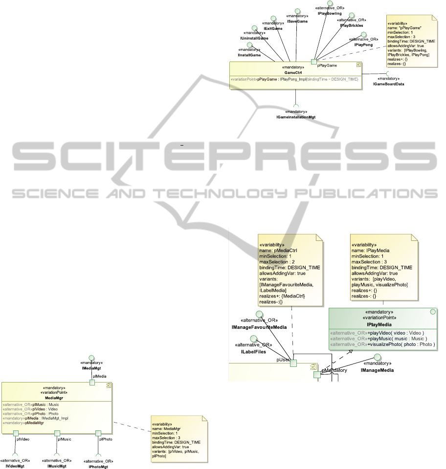
Figure 2 presents an excerpt of the Mobile Me-

dia SPLA according to SMarty 5.2. Ports pIMusic,

pIVideo and pIPhoto are inclusive variants related

to the variation point component MediaMgr. Note that

port pIMedia is mandatory for such a component.

vis´ıvel em seu compartimento, onde este indica que apenas uma destas variantes deve ser

selecionada.

Figura 3.3: Relacionamento de Componentes e Portas.

O componente MediaMgr, apresentado na Figura - 3.3, possui uma nota¸c˜ao UML

que representa as propriedades das variabilidades associadas, atrav´es do estere´otipo



variability



, onde indica as variantes relacionadas, o m´ınimo e o m´aximo de variantes

que podem ser selecionadas e o tempo de liga¸c˜ao em que as variabilidades s˜ao resolvidas.

O relacionamento com portas ´e opcional por si s´o, por´em al´em de permitir uma melhor

organiza¸c˜ao das interfaces, a utiliza¸c˜ao das portas, pode trazer benef´ıcios que envolvem

reutiliza¸c˜ao de portas e interfaces. Neste exemplo, foi utilizado as portas em interfaces

separadas somente como uma forma de representar o relacionamento de componentes e

portas, mas em exemplos pr´oximos a este, sugere o uso de somente uma porta, e esta porta

sendo um ponto de varia¸c˜ao em rela¸c˜ao as interfaces. J´a na Figura - 3.4, h´a um exemplo

mais expl´ıcito da utiliza¸c˜ao de portas, com o intuito de separar as interfaces e melhorar

seus relacionamentos, facilitando a identiﬁca¸c˜ao e representa¸c˜ao das variabilidades.

Neste exemplo, o componente MediaCtrl, retirado da Vers˜ao 8 da LPS MM (Con-

tieri Junior, 2010), apresenta uma representa¸c˜ao de variabilidades diretamente com as

portas, sendo o pr´oprio componente um ponto de varia¸c˜ao, anotado com o estere´otipo



variationPoint



e as portas pUser e pMediaCtrl como sendo suas variantes, anotadas

com o estere´otipo



alternative OR



. Al´em deste estere´otipo, ambas as portas foram

Figure 2: Mobile Media Excerpt According to SMarty 5.2:

MediaMgr Variation Point Component and Respective In-

clusive Variant Ports.

Figure 3 presents an excerpt of the Mobile Me-

dia SPLA according to SMarty 5.2. Interfaces

IPlayBowling, IPlayBrickles and IPlayPong are

inclusive variants related to the variation point port

pPlayGame, according to guideline CP.2. A spe-

ciﬁc product derived from such an excerpt must have

at least 1 (minSelection attribute) and at most 3

(maxSelection attribute) interfaces from such a port.

porta, IPlayBowling, IPlayBrickles e iPlayPong, s˜ao as respectivas variantes e est˜ao

estereotipadas como



alternative OR



Figura 3.2: Relacionamento de porta com interfaces.

Neste exemplo, a porta pPlayGame est´a atribu´ıda `as interfaces que operam a ini-

cializa¸c˜ao dos jogos, onde na vers˜ao 2 da LPS AGM proposta por (Xavier, 2011), o

componente GameCtrl foi dividido em dois, justamente para evitar a sobrecarga sobre um

componente espec´ıﬁco, e tais interfaces foram atribu´ıdas ao componente PlayGameCtrl,

que ser´a apresentado posteriormente na Figura Figura - 3.5.

3.2.3 Relacionamento Componentes e Portas

A Figura - 3.3 apresenta um exemplo de um componente de servi¸co MediaMgr, extra´ıdo

da LPS MobileMedia (Contieri Junior, 2010). Este componente tem a fun¸c˜ao de fornecer

servi¸cos que a aplica¸c˜ao pode requerer, neste caso uma m´ıdia, podendo ser um v´ıdeo,

uma m´usica ou uma foto. Desta forma, este componente ´e um ponto de varia¸c˜ao e est´a

anotado como o estere´otipo



variationPoint



, e em seu compartimento apresenta-se

vis´ıveis as portas que este componente possui. Este componente possui 4 portas, sendo a

pMedia, uma porta que fornece o servi¸co respectivo deste componente. As demais portas

(pIVideo, pIMusic e pIPhoto) que fornecem os servi¸cos espec´ıﬁcos s˜ao, respectivamente,

as variantes, e tais portas est˜ao anotadas com o estere´otipo



alternative OR



, que ´e

Figure 3: Mobile Media Excerpt According to SMarty 5.2:

pPlayGame Variation Point Port and Respective Inclusive

Variant Interfaces.

Figure 4 presents an excerpt of the Mobile Me-

dia SPLA according to SMarty 5.2. Operations

playVideo, playMusic and visualizePhoto are in-

clusive variants related to the variation point interface

IPlayMedia.

(a) (b)

Figura 3.1: Representa¸c˜ao de Variabilidades em Interfaces com Opera¸c˜oes.

varia¸c˜ao, e tais opera¸c˜oes suas respectivas variantes. Tais opera¸c˜oes foram anotadas com

o estere´otipo



alternative OR



, nas quais, atrav´es do coment´ario UML percebe-se que

no m´ınimo uma e no m´aximo trˆes das variantes devem ser selecionadas. J´a no modelo

(b) deste mesmo exemplo, ´e poss´ıvel visualizar o estere´otipo do ponto de varia¸c˜ao, por´em

suas opera¸c˜oes ﬁcam ocultas, podendo percebˆe-las somente atrav´es do item variants no

coment´ario UML ligado `a interface.

3.2.2 Relacionamento Portas e Interfaces

Existem casos espec´ıﬁcos que se sugerem o uso de portas, como por exemplo, na

Figura - 3.2, h´a um modelo em que o componente GameCtrl possui uma porta, mas

tamb´em possui interfaces diretamente relacionadas. Este modelo de componente foi

retirado da LPS AGM em sua vers˜ao 1 porposta por Correia (2010), e apresenta as

interfaces dos jogos dispon´ıveis, ligados a uma determinada porta, e interfaces das

opera¸c˜oes necess´arias do jogo, como por exemplo para instala¸c˜ao do jogo, salvar o

jogo, desinstalar o jogo e sair do jogo. Neste exemplo, foi sugerida a utiliza¸c˜ao da

porta como ponto de varia¸c˜ao, justamente para separar as interfaces que s˜ao de uma

determinada fun¸c˜ao, e que ocorrem algum tipo de variabilidade. Para a porta pPlayGame,

foi atribu´ıda a anota¸c˜ao do estere´otipo



variationPoint



representando um ponto de

varia¸c˜ao, e tal estere´otipo pode ser visualizado em seu compartimento, frente ao nome

da respectiva porta. Um coment´ario UML representando variabilidade est´a anotada

com o respectivo estere´otipo



variability



, e neste indicam quais interfaces s˜ao suas

variantes, a quantidade m´ınima e m´axima de sele¸c˜ao. As interfaces relacionadas a esta

Figure 4: Mobile Media Excerpt According to SMarty 5.2:

IPlayMedia Variation Point Interface and Respective In-

clusive Variant Operations.

4 EFFECTIVENESS OF SMarty:

EXPERIMENTAL STUDY

This section presents an experimental study in order

to compare SMarty 5.2 and the Razavian and Khos-

ravi approach with relation to their effectiveness in

identifying and representing variability in component

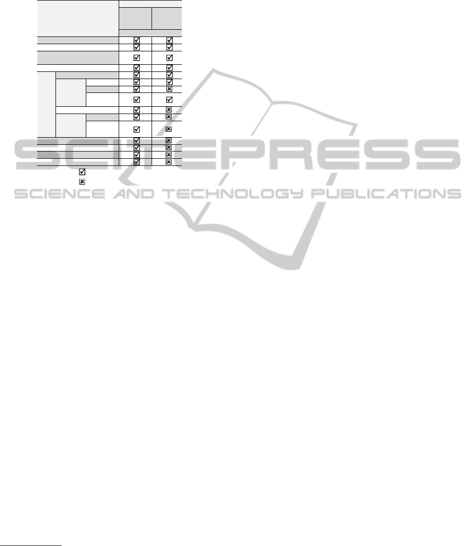
models. Table 2 summarizes the main features of such

approaches. Note that in most criteria, SMarty and the

Razavian and Khosravi approach are similar. Thus,

ICEIS2015-17thInternationalConferenceonEnterpriseInformationSystems

298

such a similarity and its popularity

justify our choice

for the Razavian and Khosravi approach.

Table 2: SMarty and Razavian and Khosravi Approaches

Support for UML Component Models.

SMarty 5.2

Razavian and

Khosravi

(Razavian and

Khosravi, 2008)

Optional

Inclusive (OR)

Exclusive

(XOR)

Complement

Mutually

Exclusive

Legend:

Does not support the criterion

Constraints

Among

Variants

Explicit Representation of

Cardinality

Binding Time declaration

Addtion of new Variants

Supports the criterion

Variability

Variant

Aproaches

Component Model

Criterion

Traceability

Support for UML Models

UML Profile Definition

Guidelines for Identification and

Representation of Variability

UML Stereotypes

Variation Point

4.1 Experiment Deﬁnition

The goal of this experiment was to compare the Raza-

vian and Khosravi and the SMarty approaches, for

the purpose of identifying the most effective, with

respect to the capability of identiﬁcation and rep-

resentation of variabilities in SPLA UML compo-

nent models, from the point of view of SPL archi-

tects, in the context of master and Ph.D. students of

the Software Engineering area from the State Uni-

versity of Maring

a (UEM), University of S

ao Paulo

(ICMC-USP) and Pontiﬁcal Catholic University of

Rio Grande do Sul (PUCRS).

It established the following research question

(R.Q.): Which methodology is more effective at iden-

tifying and representing variabilities in SPLA UML

component models: SMarty 5.2 or Razavian and

Khosravi?

4.2 Experiment Planning

Training: subjects were trained with regard to essen-

tial concepts of SPL and variability and UML compo-

nent models variability identiﬁcation and representa-

tion using the Razavian and Khosravi or SMarty ap-

proaches.

Pilot Project: it was conducted with a lecturer,

working for 25 years in the area of Software Engi-

The Razavian and Khosravi approach is cited in vari-

ous works as indicated by Google Scholar at http://scholar.

google.com/citations?user=hwtquZEAAAAJ&hl=en

neering. She provided adjustments for improving the

experiment instrumentation.

Selection of Subjects: the 14 selected subjects

were master and Ph.D. students who have prior

knowledge in UML modeling components. Further-

more, after training, each subject should be familiar

with SPL variability essential concepts.

Instrumentation: each subject was given a set of

documents, as follows:

• term of informed consent (TCLE - Brazilian stan-

dard for this type of experiment);

• a characterization questionnaire.This document

was previously ﬁlled online, then used to sepa-

rate subjects according to their prior knowledge

to avoid any biases; and

• the description of Virtual University and Mobile

Media SPLs and their component models with no

variabilities.

Balancing: subjects were separated into two

groups by their knowledge. One group focused on the

X approach (Razavian and Khosravi) and one group

focused on the Y approach (SMarty). One group was

trained to identify and represent variabilities accord-

ing to the X approach and the other group was trained

to identify and represent variabilities according to the

Y approach. Tasks were assigned in equal number to

a similar number of subjects.

Hypotheses Formulation: the following hy-

potheses were tested in this study:

Null Hypothesis (H

): both X and Y approaches

are equally effective in terms of identifying and rep-

resenting variabilities in UML component models.

Alternative Hypothesis (H

): X approach is less

effective than Y approach.

Alternative Hypothesis (H

): X approach is

more effective than Y approach.

Dependent Variable: effectiveness calculated

for a given variability management approach (X and

Y) as follows:

effectiveness(z) =

(

nVarC, if nVarI=0

nVarC − nVarI, if nVarI>0

(1)

where:

• z is a variability management approach;

• nVarC is the number of correct identiﬁed variabil-

ity elements according to the z approach;

• nVarI is the number of incorrect identiﬁed vari-

ability elements according to the z approach.

A variability element might be either a variation

point or a variant. The effectiveness expression is in-

spired in several works, including SPL, as (Basili and

Evidence-basedSMartySupportforVariabilityIdentificationandRepresentationinComponentModels

299

Selby, 1987; Coteli, 2013; Martinez-Ruiz et al., 2011;

Marcolino et al., 2014a; Marcolino et al., 2014b).

Independent Variables: the variability

management approach, which is a factor with two

treatments (X and Y) and the SPL, which is a factor

with two treatments (Virtual University and Mobile

Media). Virtual University was selected as Razavian

and Khosravi provides explanations of their approach

based on such an SPL, thus we understand that its

selection is essential. Mobile Media is a well-known

SPL, already consolidated in the SPL community.

Random Capacity: selection of the subjects was

not random within the universe of the volunteers,

which was quite restricted. The random capacity took

place at the assignment of the variability management

approach (X or Y) to each subject.

4.3 Execution

The main task for each subject was reading and un-

derstanding the Virtual University and Mobile Media

SPLs description documents, randomly distributed.

Then, subjects annotated variabilities in the SPL mod-

els.

Participation Procedure: the following proce-

dures were performed for each subject participation:

0. subjects answer an online characterization

questionnaire;

1. subject personally attended the location where

the study took place;

2. experimenter gives subject a set of documents:

(i) the experimental study consent term; (ii) document

with essential concepts of variability management in

SPL; (iii) document with essential concepts of UML

2.5; and (iv) the description of the Virtual University

and Mobile Media SPLs.

3. experimenter randomly associates each subject

to the X or Y approach;

4. experimenter trains the subjects on respective

approach;

5. subject identiﬁes and represents variabilities in

the Virtual University and Mobile Media component

models according to his/her associated approach.

Collected data is presented in Table 3 and ana-

lyzed using appropriate statistical methods, which are

properly discussed in Section 4.4. For each subject

(“Subject #” column), the following data for his/her

given approach was collected: the number of correct

and incorrect identiﬁed and represented variabilities;

and the effectiveness calculation.

Correct/Incorrect Variability Rate Criteria:

criteria was based on the variability of the Virtual Uni-

versity and Mobile Media SPLs. Each correct vari-

ability corresponds to 1 point. Each SPL has 11 vari-

abilities, thus a maximum score of 11 points is possi-

ble. Therefore, subjects had to model two SPLs with

a maximum score of 22 points.

Figure 5 presents X and Y approaches effective-

ness boxplot.

Box Plot of multiple variables

Median; Box: 25%-75%; Whisker: Non-Outlier Range

Median

25%-75%

Non-Outlier Range

Outliers

Extremes

X Approach Y Approach

-8

-6

-4

-2

Figure 5: Effectiveness of X and Y Approaches.

4.4 Analysis and Interpretation

Based on the results obtained by analyzing the ap-

plication of the X and Y approaches to the Virtual

University and Mobile Media SPLs, we analyzed and

interpreted the X and Y collected data (sample) by

means of the Shapiro-Wilk normality test and the T

Test for testing the deﬁned hypotheses.

1. Effectiveness Normality Tests: Shapiro-Wilk

test was applied to the Virtual University and Mo-

bile Media samples (Table 3) providing the fol-

lowing results:

• Effectiveness of X approach (N=7): with

a mean value (µ) 6.4286, standard deviation

value of (σ) 8.3118, the total effectiveness for X

approach was p = 0.8725 for the Shapiro-Wilk

test. Thus, for a signiﬁcance level (α = 0.05), p

= 0.8725 (0.8725 > 0.05) and calculated value

of W = 0.9665 > W = 0.8030, the sample is

considered normal.

• Effectiveness of Y Approach (N=7): with a

mean (µ) 9.2571, standard deviation (σ) 5.0089,

the total effectiveness for the Y approach was

p = 0.5797 for the Shapiro-Wilk test. Thus,

for a signiﬁcance level (α = 0.05), p = 0.5797

(0.5797 > 0.05) and calculated value W =

0.9333 > W = 0.8030, the sample is considered

normal.

2. Effectiveness Hypothesis Test: T-test was ap-

plied for samples X and Y as they are indepen-

dent.

ICEIS2015-17thInternationalConferenceonEnterpriseInformationSystems

300

Table 3: Virtual University and Mobile Media SPLs Collected Data and Descriptive Statistics for the X (Razavian and Khos-

ravi) and Y (SMarty) Approaches.

Subject#

Correct

Identified

Variabilities

Incorrect

Identified

Variabilities

Effectiveness

Calculation

Subject#

Correct

Identified

Variabilities

Incorrect

Identified

Variabilities

Effectiveness

Calculation

15.90 6.10 9.80

18.60 3.40 15.20

10.20 11.80 -1.60

15.70 6.30 9.40

17.50 4.50 13.00

15.10 6.90 8.20

19.60 2.40 17.20

14.20 8.70 6.40

15.40 6.60 8.80

12.10 9.90 2.20

13.20 8.80 4.40

14.50 7.50 7.00

7.20 13.80 -6.60

19.20 2.80 16.40

Mean

14.14

7.71

6.43

Mean

15.63 6.50 9.26

Std. Dev.

4.29

4.03

8.31

Std. Dev.

2.50 2.61 5.01

Median

15.40

6.60

8.80

Median

15.10 6.90 8.20

SW#W p StdDV SW#W p StdDV

Efetividade 0,9665 0,8725 8,3118 Efetividade 0,9333 0,5797 5,00089

Acertos 0,965 0,8603 4,2887 Acertos 0,9333 0,5797 2,5045

Erros 0,966 0,8685 4,0276 Erros 0,9397 0,6358 2,6109

The X Approach (Razavian and Khosravi) The Y Approach (SMarty 5.2)

First, the value of T was obtained, which allows

the identiﬁcation of the range entered in the sta-

tistical table T (student). This value is calculated

using the average of Sample X (µ1 = 6.4286) and

Sample Y (µ2 = 9.2571), standard deviation value

of both (σ1 = 8.3118 and σ2 = 5.0089), and the

sample sizes (N = 7). It was obtained the value

calculated

= 0.7711.

By taking the sample size (N = 7), we obtained the

degree of freedom (df ), which combined to the

t value indicates which value of p in the T table

must be selected. The p value is used to accept or

reject the T-test null hypothesis (H

By searching the index d f = 12 and deﬁning the

value t at the T table (student), it was found

a value for critical t of 2.179 (t

critical

= 2.179),

with a signiﬁcance level (α) of 0.05. This means

that the probability of t

calculated

(0.7711) < t

critical

(2.132) is 95%. Thus, the null hypothesis H

must

be rejected.

Therefore, based on the result from the T-test, the

null hypothesis (H

) of this experimental study (Sec-

tion 4.2) can be rejected. By analyzing Figure 5 it

can be observed that the Y approach (SMarty Ap-

proach) is more effective than the X approach (Raza-

vian and Khosravi Approach) for representing vari-

ability at SPL component level for this experimental

study. Thus, H

can be accepted.

Based on this analysis, we can observe that

SMarty 5.2 had a superior result corroborated by the

fact that: (i) SMarty is more precise on modeling ﬁne-

grained variability detail, such as, min and max num-

ber of variants to be selected and the set of possi-

ble variant choices, whereas the Razavian and Khos-

ravi approach has no such details; (ii) taking into

account such details, SMarty has a major capability

of deriving consistent speciﬁc products with no do-

main expert intervention; and (iii) with no domain

expert intervention, the consistent speciﬁc products

derivation process can be fully automated in SMarty,

whereas deriving products from Razavian and Khos-

ravi variability component models requires a prospec-

tive human-supervised stage as it provides insufﬁcient

information.

In a comparison between SMarty version 5.1 and

the Razavian and Khosravi approach, the later would

provide a huge effectiveness as SMarty 5.1 was in-

cipient by only tagging a component as variable

and providing no mechanism to derive speciﬁc prod-

ucts based on such a modeling. Thus, it corroborates

that SMarty needed to evolve to version 5.2.

4.5 Validity Evaluation

Threats to Conclusion Validity. Sample size (N=14)

was too small, thus it must be increased in prospective

replications.

Threats to Construct Validity. Construction of

the experiment was based on the characteristics of

each SPL, and instrumentation evaluated during the

pilot project.

Threats to Internal Validity. Subject knowledge

was prior balanced, to perform the experiment tasks,

based on the characterization questionnaire to avoid

biases in random block division. Training and experi-

ment sessions were performed in different days, with

an average of 30 minutes each, thus fatigue was not

considered relevant. Subjects were supervised by a

human, thus they did not talk to each other before and

during the experiment sessions.

Threats to External Validity. Component mod-

els of the SPLs are not commercial, thus further stud-

ies must consider real SPLs. Although masters and

Ph.D. students were selected rather than practitioners

from industry, they were not considered a bias to this

study as the importance of using students in experi-

mental studies (H

ost et al., 2000).

5 CONCLUSION AND FUTURE

WORK

This paper presented an improved version of the

Evidence-basedSMartySupportforVariabilityIdentificationandRepresentationinComponentModels

301

SMarty approach to represent variability in UML

components models, speciﬁcally at four levels: (i)

components; (ii) ports; (iii) interfaces; and (iv) inter-

face operations.

Furthermore, this paper also presented an exper-

imental study performed with the goal of observing

the effectiveness of SMarty. This experimental study

was conducted based on the comparison of two ap-

proaches, SMarty 5.2 and Razavian and Kosravi, to

represent variabilities in SPL components. The re-

sults provide evidence of the effectiveness of SMarty

approach to model variability in UML components

models, in the context of the performed study.

Given the promising results, new experimental

studies and replications should be conducted. Such

further studies should take into consideration some is-

sues such as real SPLs; industry subjects in order to

generalize the results expected; and the increase of the

sample. Such considerations are important in order to

corroborate the results of this experimental study.

ACKNOWLEDGEMENTS

The authors thank CAPES-Brasil for granting M.

Bera a two-year masters degree scholarship.

REFERENCES

Basili, V. and Selby, R. (1987). Comparing the Effec-

tiveness of Software Testing Strategies. IEEE Trans-

actions on Software Engineering, SE-13(12):1278–

1296.

Capilla, R., Bosch, J., and Kang, K.-C. (2013). Systems and

Software Variability Management - Concepts, Tools

and Experiences. Springer, New York, NY, USA.

Choi, Y., Shin, G., Yang, Y., and Park, C. (2005). An

Approach to Extension of UML 2.0 for Representing

Variabilities. In ICIS, pages 258–261.

Coteli, M. B. (2013). Testing Effectiveness and Effort in

Software Product Lines. Master’s thesis, Middle East

Technical University.

Galster, M., Weyns, D., Tofan, D., Michalik, B., and Avge-

riou, P. (2014). Variability in Software Systems - a

Systematic Literature Review. IEEE Transactions on

Software Engineering, 40(3):282–306.

Gomaa, H. (2013). Evolving Software Requirements and

Architectures Using Software Product Line Concepts.

In Int. Workshop on the Twin Peaks of Requirements

and Architecture, pages 24–28.

ost, M., Regnell, B., and Wohlin, C. (2000). Using Stu-

dents As Subjects: a Comparative Study of Students

and Professionals in Lead-Time Impact Assessment.

Empirical Software Engineering, 5(3):201–214.

Ivers, J., Clements, P. C., Garlan, D., Nord, R., Schmerl, B.,

and Silva, O. (2004). Documenting Component and

Connector Views with UML 2.0. Technical report,

School of Comp. Science, Carnegie Mellon Univ.

Jazayeri, M., Ran, A., and van der Linden, F. (2000). Soft-

ware Architecture for Product Families: Principles

and Practice. Addison-Wesley Longman Publishing

Co., Inc., Boston, MA, USA.

Linden, F. J. v. d., Schmid, K., and Rommes, E. (2007).

Software Product Lines in Action: The Best Indus-

trial Practice in Product Line Engineering. Springer-

Verlag New York, Inc., Secaucus, NJ, USA.

Marcolino, A., OliveiraJr, E., and Gimenes, I. (2014a). To-

wards the Effectiveness of the SMarty Approach for

Variability Management at Sequence Diagram Level.

In ICEIS, pages 249–256, Lisboa, Portugal.

Marcolino, A., OliveiraJr, E., Gimenes, I., and Barbosa, E.

(2014b). Empirically Based Evolution of a Variabil-

ity Management Approach at UML Class Level. In

COMPSAC, pages 354–363, Vasteras, Sweden.

Marcolino, A., OliveiraJr, E., Gimenes, I. M. S., and Mal-

donado, J. C. (2013). Towards the Effectiveness of a

Variability Management Approach at Use Case Level.

In SEKE, pages 214–219.

Martinez-Ruiz, T., Garcia, F., Piattini, M., and M

unch, J.

(2011). Modelling Software Process Variability: an

Empirical Study. IET Software, 5(2):172–187.

OliveiraJr, E., Gimenes, I., and Maldonado, J. (2010).

Systematic Management of Variability in UML-based

Software Product Lines. Journal of Universal Com-

puter Science (JUCS), 16(17):2374–2393.

OliveiraJr, E., Gimenes, I. M. S., Maldonado, J. C.,

Masiero, P. C., and Barroca, L. (2013). Systematic

Evaluation of Software Product Line Architectures.

Journal of Universal Computer Science, 19(1):25–52.

OMG (2014). OMG Uniﬁed Modeling Language: Ver-

sion 2.5 - Beta 2. http://www.omg.org/spec/UML/

2.5/Beta2.

Pohl, K., Bockle, G., and Linden, F. (2005). Software Prod-

uct Line Engineering - Foundations, Principle, and

Techniques. Secaucus, NJ, USA: Springer-Verlag.

Razavian, M. and Khosravi, R. (2008). Modeling Variabil-

ity in the Component and Connector View of Archi-

tecture Using UML. In AICCSA, pages 801–809.

Ryu, D., Lee, D., and Baik, J. (2012). Designing an Archi-

tecture of SNS Platform by Applying a Product Line

Engineering Approach. In ICIS, pages 559–564.

Satyananda, T. K., Lee, D., Kang, S., and Hashmi, S. I.

(2007). Identifying Traceability Between Feature

Model and Software Architecture in Software Product

Line Using Formal Concept Analysis. In Int. Conf.

Computational Science and its Applications, pages

380–388, Washington, DC, USA. IEEE Computer So-

ciety.

Tekinerdogan, B. and S

ozer, H. (2012). Variability View-

point for Introducing Variability in Software Archi-

tecture Viewpoints. In WICSA/ECSA, pages 163–166,

New York, NY, USA. ACM.

ICEIS2015-17thInternationalConferenceonEnterpriseInformationSystems

302