
Efficient Soft-output Detectors
Multi-core and GPU implementations in MIMOPack Library
Carla Ramiro S
´
anchez
1
, Antonio M. Vidal Maci
´
a
1
and Alberto Gonzalez Salvador
2
1
Department of Information Systems and Computation, Universitat Polit
`
ecnica de Val
`
encia,
Camino de Vera s/n, Valencia, Spain
2
Institute of Telecommunications and Multimedia Applications, Universitat Polit `ecnica de Val`encia,
Camino de Vera s/n, Valencia, Spain
Keywords:
Soft-output Detector, BICM, HPC Library, GPU, Multi-core, CUDA, MIMO.
Abstract:
Error control coding ensures the desired quality of service for a given data rate and is necessary to improve re-
laibility of Multiple-Input Multiple-Output (MIMO) communication systems. Therefore, a good combination
of detection MIMO schemes and coding schemes has drawn attention in recent years. The most promising
coding schemes are Bit-Interleaved Coded Modulation (BICM). At the transmitter the information bits are
encoded using an error-correction code. The soft demodulator provides the reliability information in form of
real valued log-likehood ratios (LLR). These values are used by the channel decoder to make final decisions on
the transmitted coded bits. Nevertheless, these sophisticated techniques produce a significant increase in the
computational cost and require large computational power. This paper presents a set of Soft-Output detectors
implemented in CUDA and OpenMP, which allows to considerably decrease the computational time required
for the data detection stage in MIMO systems. These detectors will be included in the future MIMOPack
library, a High Performance Computing (HPC) library for MIMO Communication Systems. Experimental re-
sults confirm that these implementations allow to accelerate the data detection stage for different constellation
sizes and number of antennas.
1 INTRODUCTION
Multiple-input multiple-output (MIMO) systems can
provide high spectral efficiency by means of spatially
multiplexing multiple data streams (Paulraj et al.,
2004), which makes them promising for current wire-
less standards. However, the use of MIMO technolo-
gies involves an increment of the detection process
complexity. The detector is present at the receiver
side and is the responsible for recover the received
signals (which are affected by the channel fluctua-
tion) with the maximum reliability. This step be-
comes in many cases the most complex stage in the
communication. Another important factor that affects
the performance of a MIMO system is the number
of transmit and receive antennas, because as the sys-
tem grows the communication process becomes more
complicated. Although the number of antennas cur-
rently allowed in the standards is not large, it is ex-
pected that in the near future more than 100 transmit
antennas will be used (Rusek et al., 2013). Thus, the
search for high-throughput practical implementations
that are also scalable with the system size is impera-
tive.
Graphic processing units (GPUs) have been
recently used to develop reconfigurable software
defined-radio platforms (Kim et al., 2010), high-
throughput MIMO detectors (Wu et al., 2010),
and fast low-density parity-check decoders (Falcao
et al., 2009). Although multicore central pro-
cessing unit (CPU) implementation could also re-
place traditional use of digital signal processors and
field-programmable gate arrays (FPGAs), this option
would interfere with the execution of the tasks as-
signed to the CPU of the computer, possibly caus-
ing speed decrease. Since the GPU is more rarely
used than the CPU in conventional applications, its
use as a coprocessor in signal-processing systems is
very promising. Therefore, systems formed by a mul-
ticore computer with one or more GPUs are interest-
ing in this context.
In this paper, we consider the use of MIMO
with bit-interleaved coded modulation (BICM) (Caire
et al., 1998). The use of these kind of system al-
lows to improve the reliability of the MIMO systems.
However, the receiver stage becomes more compli-
335
Ramiro Sánchez C., M. Vidal Maciá A. and Gonzalez Salvador A..
Efficient Soft-output Detectors - Multi-core and GPU implementations in MIMOPack Library.
DOI: 10.5220/0005369503350344
In Proceedings of the 5th International Conference on Pervasive and Embedded Computing and Communication Systems (AMC-2015), pages 335-344
ISBN: 978-989-758-084-0
Copyright
c
2015 SCITEPRESS (Science and Technology Publications, Lda.)

cated since the demodulator must to generate soft-
information (log-likehood ratios) that can be used by
the decoder. In order to accelerate the computation
of the log-likehood ratios (LLR), we present a set
of efficient soft-output decoders with different com-
plexities and performances in terms of Bit Error Rate
(BER). These soft-output detectors will be included in
the MIMOPack library and have been implemented to
be run in a multicore and GPU system. Speedup re-
sults show how the execution time of the detection
stage can be meaningfully decreased using these im-
plementations.
2 SOFT-OUTPUT MIMO
DETECTION
Let us consider a MIMO-BICM system with n
T
trans-
mit antennas and n
R
≥ n
T
receive antennas (see Fig.
1). We assume a spatial multiplexing system, where
for any time instant n, the ith data stream s
i
[n] is
transmitted on the ith transmit antenna. The base-
band equivalent model for the received vector y[n] =
(y
1
[n], ..., y
n
R
[n])
T
is given by
y[n] = H[n]s[n] +v[n], n = 1, . . . , N
c
−1, (1)
where N
c
is the number of time instants in the en-
tire transmission. H[n] is an n
R
×n
T
matrix model-
ing the Rayleigh fading MIMO channel, and the noise
components of vector v[n] = (v
1
[n], ..., v
n
R
[n])
T
are
assumed independent and circularly symmetric com-
plex Gaussian with variance σ
2
w
. We assume that the
channel H[n] is known at the receiver and the symbols
are taken from a constellation Ω of size |Ω|= 2
m
= M.
For the sake of simplicity, we will omit the time index
n and, thus write (1) as
y = Hs +v. (2)
In this system, the sequence of information bits b
is encoded using an error correcting code before being
demultiplexed into n
T
layers. The coded bits are then
passed through an interleaver Π and mapped via Gray
labeling.
At the receiver side, the demodulator uses the
model (1) to calculate the soft information about the
code bits in terms of log-likelihood ratios LLRs (Λ).
Thus, to calculate an Λ
i,k
for each coded bit b
i,k
, with
k = 1, . . . ,m, of the sent symbol vector s, the detector
uses the received vector y and the channel matrix H.
Finally, the reliability information is de-interleaved
(Π
−1
) and multiplexed into a single stream which will
be used by the channel decoder.
A strategy to decrease slightly the complexity of
the detection is to reduce the channel matrix in a
canonical form by orthogonal transformations before
the detection. If QR decomposition is employed in
a preprocessing stage, the channel matrix is decom-
posed into H = QR, where R is an upper triangu-
lar matrix. Left-multiplying (2) by Q
H
and calling
˜
y = Q
H
y, the problem can be rewritten as:
ˆ
s = arg min
s∈Ω
n
T
kQ
H
y −Rsk
2
= arg min
s∈Ω
n
T
k
˜
y −Rsk
2
,
(3)
where the most probable transmitted symbol vector
ˆ
s
is found by searching the smallest distance between
the received vector y and each possible vector s. To
clarify how the triangular structure of R can be ex-
ploited, Eq. 3 has been expressed in a more explicit
way
ˆ
s = arg min
x∈Ω
n
T
1
∑
i=n
T
˜y
i
−
n
T
∑
j=i
R
i j
s
j
2
. (4)
Problem (4) can be represented as a decoding tree
with n
T
+ 1 levels. Each possible message s is repre-
sented by a branch and each symbol value by a node.
Then there are M
n
T
leaf nodes which represent the to-
tal of possible values for s. In order to solve Eq. 4 via
tree search, the following recursion is performed for
i = n
T
, n
T
−1, . . . , 1 :
D
i
(S
i
) = D
i+1
(S
i+1
) + |e
i
(S
i
)|
2
, (5)
where i denotes each tree level, S
(i)
=
[s
i
, s
i+1
, . . . , s
n
T
], D
i
(S
(i)
) is the accumulated Par-
tial Euclidean Distance (PED) up to level i, with
D
n
T
+1
(S
n
T
+1
) is set to 0 and the Distance Increment
(DI), also called branch weight is computed as:
e
i
(S
i
) = ˜y
i
−
n
T
∑
j=i
R
i j
s
j
. (6)
3 TOOLS AND OPTIMIZATION
TECHNIQUES
In this section we present some tools and additional
optimizations performed to accelerate and reduce the
number of FLOPS (floating points operations) needed
to perform the detection. These strategies will be used
in many of the algorithms and therefore are needed to
understand the implementations in the next section.
PECCS2015-5thInternationalConferenceonPervasiveandEmbeddedComputingandCommunicationSystems
336
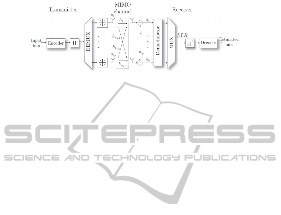
Figure 1: Block diagram of a MIMO-BICM system.
3.1 Graphic Processing Units and
CUDA
Compute Unified Device Architecture (CUDA)
(NVIDIA, 2014) is a software programming model
that exploits the massive computation potential of-
fered by GPUs. A GPU can have multiple stream
multiprocessors (SM), each with a certain number of
pipelined cores. A CUDA device has a large amount
of off-chip device memory (global memory) and a fast
on-chip memory called shared memory. Following
Flynn’s taxonomy (Flynn, 1972), from a conceptual
point of view, a GPU can be considered as a single
instruction, multiple data (SIMD) machine; that is, a
device in which a single set of instructions is executed
on different data sets. In the CUDA model, the pro-
grammer defines the kernel function which contains
a set of common operations. At runtime, the kernel
is called from the main central processing unit (CPU)
and spawns a large number of threads blocks, which
is called a grid. Each thread block contains multiple
threads and all the blocks within a grid must have the
same size. Each thread can select a set of data using
its own unique ID and execute the kernel function on
the selected set of data. Threads within a block can
synchronize their execution through a barrier to co-
ordinate memory accesses. In contrast, thread blocks
are completely independent and can only share data
through the global memory once the kernel ends.
3.2 Multicore Processors and OpenMP
OpenMP is an Application Programming Interface
(API) (OpenMP, 2013) for programming shared-
memory parallel computers. It consists of a set of
compiler directives, callable library routines and en-
vironment variables which may be embedded within
a code written in a programming language such as
Fortran, C/C++ on several processor architectures and
operating systems such as GNU/Linux, Mac OS X,
and Windows platforms.
Basically, a master thread launch a number of
slave threads and divide the workload among them.
The runtime will attempt to allocate the threads to
different processors and the threads will run concur-
rently.
The multicore parallelization performed in the
Soft-Output detectors is common for all of them and
is based in the estimation of a particular transmitted
signal
ˆ
s[n] per thread.
3.3 Efficient Calculation of Partial
Euclidean Distances
We propose a strategy, consisting in the previous es-
timation of all posible values of the inner sumatory
∑
n
T
j=i
R
i j
s
j
in equation (4). This will allow us to avoid
common computation for different possible solutions
(s ∈ Ω
n
T
) decreassing the computational cost of the
detection process. These values are stored in a M ×n
v
matrix T. The elements T
i, j
, contains the result of
multiplying the constellation symbol Ω
i
by the j-th
non-zero value of matrix R:
T =
Ω
1
R
1,1
Ω
1
R
1,2
. . . Ω
1
R
n
T
,n
T
Ω
2
R
1,1
Ω
2
R
1,2
. . . Ω
2
R
n
T
,n
T
.
.
.
.
.
.
.
.
.
.
.
.
Ω
M
R
1,1
Ω
M
R
1,2
. . . Ω
M
R
n
T
,n
T
, (7)
where n
v
is the number of non-zero values of R.
Then, each row i contains all non-zero valued el-
ements of matrix R multiplied by the constellation
complex-valued symbol Ω
i
.
Algorithm 1 shows the steps needed to calculate
the accumulated PED of a path s from the root up to
level lini by using the matrix T. As an example, let us
consider a 2 ×2 MIMO system using a 16-QAM con-
stellation, which has the following triangular matrix
associated
R =
R
1
1,1
R
2
1,2
0 R
3
2,2
,
the n
v
= 3 non-zero values are represented as R
(l)
i, j
,
where l represents the index of the column that it oc-
EfficientSoft-outputDetectors-Multi-coreandGPUimplementationsinMIMOPackLibrary
337

cupies in the T matrix. We want to calculate the Par-
tial Euclidean Distances (PED) of the following tree-
path S:
S
(1)
= [s
1
, s
2
]
T
= [−3 −1i, 1 −3i]
T
= [Ω
3
, Ω
15
]
T
,
the Distance Increment (DI) are computed as follows:
e
2
(S
(2)
) = ˜y
2
−
n
T
∑
j=2
R
i, j
s
j
= ˜y
2
−R
2,2
Ω
15
= ˜y
2
−T
15,3
(8)
e
1
(S
(1)
) = ˜y
1
−
n
T
∑
j=1
R
i, j
s
j
= ˜y
1
−(R
1,1
Ω
3
+ R
1,2
Ω
15
)
= ˜y
1
−(T
3,1
+ T
15,2
)
(9)
Assuming that the root node starts with accumu-
lated PED equal to zero d
3
(S
(3)
) = 0; the final Eu-
clidean Distance at the leaf node is:
d
1
(S
(1)
) = |˜y
2
−T
15,3
|
2
+ |˜y
1
−(T
3,1
+ T
15,2
)|
2
(10)
Algorithm 1: Efficient Calculation of Accumulated
Partial Euclidean Distances from level lini to lend.
Input: T,
˜
y, s
Output: D
lini
1: D
n
T
+1
= 0
2: for i = n
T
, . . . , lini do
3: for j = i, . . . , n
T
do
4: Get index l using i and j,
5: aux = aux + T
s
j
,l
6: end for
7: D
i
= D
i+1
+ |˜y
i
−aux|
2
8: end for
4 SOFT-OUTPUT DETECTORS
IMPLEMENTATION
4.1 Optimum and Max-log
Demodulators
Assuming that all transmit vectors are equally likely
the optimal soft MAP (OMAP) demodulator calcu-
lates the exact LLR for b
i,k
as
Λ
i,k
= log
P(b
i,k
= 1|y, H)
P(b
i,k
= 0|y, H)
= log
∑
s:s
i
∈Ω
1
k
e
−
k
˜
y−Rs
k
2
σ
2
w
∑
s:s
i
∈Ω
0
k
e
−
k
˜
y−Rs
k
2
σ
2
w
(11)
where Ω
u
k
denotes the set of all symbols s ∈ Ω whose
label u ∈ {0, 1} in bit position k. The complexity of
this method is O(|Ω|
n
T
) since the LLRs are calculated
for all layers n
T
, therefore is mandatory the computa-
tion of |Ω|
n
T
distances.
If the receiver uses a max-log approximation
(MLA) demodulation the computation of the LLRs
for each code bit is calculed according to (Muller-
Weinfurtner, 2002)
Λ
i,k
≈
1
σ
2
w
"
min
s:s
i
∈Ω
0
k
k
˜
y −Rs
k
2
− min
s:s
i
∈Ω
1
k
k
˜
y −Rs
k
2
#
.
(12)
There are numerous suboptimal alternatives of
soft MIMO detectors in order to avoid an exhaus-
tive search over the entire range of possibilities |Ω|
n
T
.
In this paper two tree-search-based soft demodulation
have been considered and are described in future sec-
tions.
4.1.1 CUDA Implementation
The proposed OMAP and MLA GPU implementa-
tions have a similar algorithmic scheme. Both CUDA
codes are composed by two kernels which work to-
gether to perform the estimation of the signals re-
ceived in N
c
time slots.
Algorithm 2: CUDA Parallelization for the OMAP
and MLA detection of N
c
time instants.
1: Allocate Memory in GPU-GM for: T,
˜
y, s and D,
2: Copy from CPU to GPU-GM: T and
˜
y,
3: Copy from CPU to GPU Constant Memory: gray,
4: Select kernel configuration with n
th
= N
c
·M
n
T
,
5: Obtain D and s using Kernel 1
6: Select kernel configuration with n
th
= N
c
·m ·n
T
7: if OMAP method is selected then
8: Obtain Λ using Kernel 2
9: else
10: Obtain Λ using Kernel 3
11: end if
12: Copy from GPU-GM to CPU: Λ
Algorithm 2 shows the steps needed to launch the
kernel. First, is necessary to allocate memory in the
GPU Global Memory (GPU-GM) for input (T,
˜
y),
output (D) and auxiliary (s) matrices related to the N
c
signals. Then, input matrices should be copied into
the GPU-GM. The next step is to launch the Kernel 1,
with the appropiatte grid dimension.
In Kernel 1, each thread is in charge to compute
the accumulated PED for a given signal n and a pos-
sible jth combination of the range Ω
n
T
. During the
detection process, the detector should maintain a list
of P = M
n
T
symbols that are being estimated for each
PECCS2015-5thInternationalConferenceonPervasiveandEmbeddedComputingandCommunicationSystems
338

signal. In order to reduce memory requirements and
the cost of data transfers our algorithms keep the list
of symbols in integer format (not complex) which will
be represented as s
:, j
. This is especially important for
the GPU implementations since they have certain lim-
its in memory capacity and the data transfers to/from
the CPU are very expensive. Once the indices of the
constellation symbols for a given three-path j have
been obtained (see step 3) , its Euclidean Distance
is calculated by adding different elements of the pre-
built matrix T such as Alg. 1 and store it in D
j
[n].
Therefore n
th
= N
c
·M
n
T
threads are needed to
launch the kernel. A bidimensional grid configura-
tion with N
Bx
= N
B
, N
By
= N
B
has been considered
for all Soft Detectors. The number of blocks N
B
de-
pends on the number of threads per dimension, which
are denoted by N
tx
and N
ty
, respectively. The block
size will be chosen to be a multiple of 32 in order to
avoid incomplete warps. Then the value of N
B
is ob-
tained as:
N
B
=
r
n
th
(N
tx
·N
ty
)
. (13)
Kernel 1: Calculation of one of the branches of the
OMAP and MLA detectors by the z-th thread for N
c
time slots.
Input: T,
˜
y, N
c
Output: D, s
1: Calculate using the thread global index z:
• Time slot identifier n
• Path identifier j
2: if n < N
c
then
3: Get selected path s
:, j
[n],
4: Compute Euclidean Distance D
j
[n] from 1 to n
T
level using T[n] and
˜
y[n]
5: end if
Once the Euclidean Distances have been calcu-
lated the detector must to obtain the soft information.
Depending on the kind of detector selected (OMAP
or MLA) Kernel 2 or Kernel 3 will be launched.
In this case the number of blocks is computed as
Eq.13 with n
th
= N
c
· m · n
T
. Each thread is in
charge to compute an LLR Λ
i,k
for a determinated
time index n using Eq.11 or Eq.12 respectively. A
matrix, called gray of size M ×m, is used in order
to find the set of symbols Ω
u
k
with k = 1, . . . , m
. This matrix contains the representation of all
constellation symbols in binary format. This data
will not change during the execution and is read only,
then its very suitable to be copied in constant memory.
Kernel 2: Computation of the LLR for the OMAP by
the z-th thread for N
c
time slots.
Input: D, s, N
c
, σ
2
w
Output: Λ
1: Calculate using the thread global index z:
• Time slot identifier n
• Layer position i
• Bit position k
2: Set d0 = 0 and d1 = 0
3: if n < N
c
then
4: for j = 1, . . . , P do
5: Get ith symbol s = s
i, j
[n]
6: if gray
s,k
= 1 then
7: d1 = d1 +e
−
D
j
[n]
σ
2
w
8: else
9: d0 = d0 +e
−
D
j
[n]
σ
2
w
10: end if
11: end for
12: Λ
i,k
[n] = log(
d1
d0
)
13: end if
Kernel 3: Computation of the LLR for the MLA by
the z-th thread for N
c
time slots.
Input: D, s, N
c
, σ
2
w
Output: Λ
1: Calculate using the thread global index z:
• Time slot identifier n
• Layer position i
• Bit position k
2: Set d0 = 1e6 and d1 = 1e6
3: if n < N
c
then
4: for j = 1, . . . , P do
5: Get the ith symbol s = s
i, j
[n]
6: if gray
s,k
= 1 and D
j
[n] < d
1
then
7: d1 = D
j
[n]
8: end if
9: if gray
s,k
= 0 and D
j
[n] < d
0
then
10: d0 = D
j
[n]
11: end if
12: end for
13: Λ
i,k
[n] =
d0−d1
σ
2
w
14: end if
4.2 Soft Fixed Sphere Decoder
The Soft Fixed Sphere Decoder (SFSD) performs a
predeterminated tree-search composed of tree differ-
ent stages. The first two stages (FE and SE) are known
as the hard-output stage or HFSD detection (Barbero
and Thompson, 2008):
• A full expansion of the tree (FE) in the first (high-
est) L levels. At the FE stage, for each survivor
path, all the possible values of the constellation
are assigned to the symbol at the current level.
EfficientSoft-outputDetectors-Multi-coreandGPUimplementationsinMIMOPackLibrary
339

• A single-path expansion (SE) in the remaining
tree-levels n
T
− L. The SE stage starts from
each retained path and proceeds down in the
tree calculating the solution of the remaining
succesive-interference-cancellation (SIC) prob-
lem (Berenguer and Wang, 2003) as:
ˆs
i
= Q
(
˜y
i
−
∑
n
T
j=i+1
R
i j
ˆs
j
R
ii
)
, i = n
T
, . . . , 1.
(14)
The function Q (·) assigns the closest constella-
tion value. Note that, the efficient PED calcula-
tion using matrix T can also be used to accelerate
the computation of the sumatory
∑
n
T
j=i+1
R
i j
ˆs
j
in
the SIC problem. The symbols are detected fol-
lowing a specific ordering also proposed by the
authors in (Barbero and Thompson, 2008). As it
was shown in (Jalden et al., 2009), the maximum
detection diversity can be achieved with the FSD
if the following value of L is chose:
L ≥
√
n
T
−1 (15)
• A Soft-Output extension (SOE) to provide soft in-
formation by obtaining an improved list of candi-
dates (Barbero et al., 2008). Figure 2(b) shows
the search-tree of the SFSD for the case with
n
T
= 4 and QPSK symbols. The method starts
from the list of candidates that the hard-output
FSD in (composed by the FE and SE stages) ob-
tains (in Fig. 2(a)) and adds new candidates to
provide more information about the counter bits.
Note that, since the first level of the HFSD tree is
already totally expanded, all the necessary values
to compute the LLRs of the symbol bits in the first
levels are available. Therefore, the list extension
must start from the second level of such path. To
begin the list extension, the best N
iter
paths are se-
lected from the initial hard-ouput FSD list (in this
example, N
iter
= 2). This is based on the heuris-
tics that the lowest-distance paths may be candi-
dates differing from the best paths in only some
bits. The symbols belonging to these N
iter
paths
are picked up from the root up to a certain level l,
and, at level l −1, additional log
2
M branches are
explored, each of them having one of the bits of
the initial path symbol negated. Afterwards, these
new partial paths are completed following the SIC
path, as done in the hard-ouput FSD scheme. The
same operation is repeated until the lowest level
of the tree is reached.
Figure 2: Decoding trees of the SFSD algorithm for a 4 ×4
MIMO system with QPSK symbols, N
iter
= 2 and L = 1: (a)
Hard-Output stage and (b) Soft-Output Extension.
4.2.1 SFSD CUDA Implementation
Algorithm 3 shows the steps needed to perform the
SFSD detection. First, data for input and output
variables are allocated and copied into the GPU-GM
memory. In this case, matrices gray, neg and constel-
lation symbols Ω are copied into constant memory.
The Ω variable is needed to perform the quantization
Q (·) in the SIC problem. Matrices D and s contains
the information of the P = M
L
+ N
iter
·m ·(n
T
−L)
paths computed: M
L
branches of the Hard-Output
stage and the N
iter
·m ·(n
T
−L) new branches of the
Soft-Output extension (SOE) stage.
In Kernel 4, each thread calculates one of the M
L
branches of the HFSD stage. After the hard-output
part is finished, the CPU is in charge to calculate the
N
iter
minimum distances and store it in the matrix min
in ascendent order. This matrix is copied in the GPU
global memory. Then, the N
iter
·m ·(n
T
−L) new can-
didates to be obtained per time index n are equally dis-
tributed among all the threads of the grid using Ker-
nel 5. As mentioned, in the SOE stage, adittional m
branches are explored in the remaining (n
T
−L) lev-
els. Each of them have one of the bits of the initial
path symbol negated. In order to accelerate this ex-
pansion, a matrix (neg) is builded before the detec-
tion. This matrix contains, for each constellation sym-
bol Ω
i
, a list of m constellations symbols resulting of
the kth bit negation. For example using QPSK con-
PECCS2015-5thInternationalConferenceonPervasiveandEmbeddedComputingandCommunicationSystems
340

Kernel 3: CUDA Parallelization for the SFSD detec-
tion of N
c
time instants.
1: Allocate Memory in GPU-GM for: T,
˜
y, s and D,
2: Copy from CPU to GPU-GM: T and
˜
y,
3: Copy from CPU to GPU Constant Memory: gray, gray
and Ω,
4: Select kernel configuration with n
th
= N
c
·M
L
,
5: HFSD Stage: Obtain D and s using Kernel 4,
6: Copy from GPU-GM to CPU: D,
7: Obtain min calculating the path indices of the N
iter
minimum distances,
8: Copy from CPU to GPU: min,
9: Select kernel configuration with n
th
= N
c
·M ·m ·(n
T
−
L),
10: SOE Stage: Update D and s using Kernel 5,
11: Select the kernel configuration with n
th
= m ·n
T
,
12: Obtain Λ using Kernel 6,
13: Copy from GPU-GM to CPU: Λ
stellation for the symbol Ω
3
its binary representation
is 11. Negating the 1st bit it becomes in 1
¯
1 = 10, then
neg
3,1
= 2, negating the 2nd bit it becomes in
¯
11 = 01,
then neg
3,2
= 1. As occurs with matrix gray, this ma-
trix is constant for the entire simulation, then will be
copied also in constant memory.
Kernel 4: Calculation of one of the branches of the
HFSD detector by the z-th thread for N
c
time slots.
Input: T,
˜
y, n
T
, N
c
, L
Output: D, s
1: Calculate using the thread global index z:
• Time slot identifier n
• Path identifier j
2: if n < N
c
then
3: Get Path from level n
T
− L + 1 to n
T
as
s
n
T
−L+1:n
T
, j
[n],
4: Compute Partial Distance D
j
[n] from n
T
−L + 1 to
n
T
level using T[n] and
˜
y[n]
5: for r = n
T
−L, . . . , 1 do
6: Compute s
r, j
[n] using SIC Eq.14,
7: Update path distance D
j
[n] using T[n] and
˜
y[n]
8: end for
9: end if
After this, the final step finds within this list the
minimum distances of paths having the counter bits
and computes the log
2
M ·n
T
LLRs. These operations
are executed by the Kernel 6.
4.3 Fully Parallel Fixed Sphere Decoder
In SFSD detector, a smart list extension based on
the lowest distance paths within the initial FSD list
is proposed, however, such extension is performed in
an almost totally sequential way, which alters the al-
gorithm parallelism degree. For this reason, a soft-
Kernel 5: Calculation of new candidates for the SFSD
detector by the z-th thread for N
c
time slots.
Input: T,
˜
y, s, min, n
T
, N
c
Output: D, s
1: Calculate using the thread global index z:
• Time slot identifier n
• Path identifier j
• Selected path N
it
• Layer position l
• Bit position k
2: if n < N
c
then
3: Get index of the selected path j
0
= min
N
it
[n],
4: and its symbol on the ith layer as s
0
= s
l, j
0
[n],
5: Copy symbols from level l to n
T
from global mem-
ory s
l+1:n
T
, j
[n] = s
l+1:n
T
, j
0
[n],
6: Get negate kth negated symbol from constant mem-
ory s
l, j
[n] = neg
s
0
[n],k
,
7: Compute partial distance D
j
[n] from l to n
T
level
8: for r = l −1,. . . , 1 do
9: Compute s
r, j
[n] using SIC Eq.(14),
10: Update path distance D
j
[n] using T[n] and
˜
y[n]
11: end for
12: end if
Kernel 6: Computation of the LLR for the SFSD by
the z-th thread for N
c
time slots.
Input: D, s, min, N
c
, σ
2
w
Output: Λ
1: Calculate using the thread global index z:
• Time slot identifier n
• Layer position i
• Bit position k
2: Set d0 = 1e6 and d1 = 1e6
3: if n < N
c
then
4: Get index of the HFSD Solution as j
0
= min
1
[n],
5: and its symbol on the ith layer as s
0
= s
i, j
0
[n],
6: for j = 1, . . . , P do
7: s = s
i, j
[n]
8: if D
j
[n] < d
min
and gray
s,k
6= gray
s
0
,k
then
9: d
min
= D
j
[n]
10: end if
11: end for
12: Λ
i,k
[n] =
(D
j
0
[n]−d
min
)(1−2gray
s
0
,k
)
σ
2
w
13: end if
output demodulator was proposed in (Roger et al.,
2012) that performs a fully parallel list extension: the
fully parallel FSD (FPFSD). The proposed approach
is purely based on the hard-output FSD scheme.
The list of candidates and distances necessary to
obtain soft information is calculated through n
T
hard-
output FSD searches, each with a different channel
matrix ordering. The n
T
different channel orderings
ensure that a different layer (level) of the system is
placed at the top of the tree each time. This way, can-
didate paths containing all the bit labelling possibili-
EfficientSoft-outputDetectors-Multi-coreandGPUimplementationsinMIMOPackLibrary
341

Table 1: Symbol detection position and corresponding tree-level for the involved FPFSD orderings in an example with n
T
= 4.
Detection Norm-based Order Order Order Order
position Ordering 1 2 3 4
1st 2 1 2 3 4
2nd 4 2 4 2 2
3rd 3 4 3 4 3
4th 1 3 1 1 1
ties in every level are guaranteed and, thus, soft infor-
mation about all the bit positions is always available.
Recall that, for n
T
= 4, 4 hard-output FSD indepen-
dent searches such as the one in Fig. 2(a) should be
carried out, each with a different channel matrix or-
dering. These tree-searches can be carried out totally
in parallel.
Note that, as when using the FSD ordering, the re-
liability of the symbol placed in the FE stage is irrel-
evant. Then, the remaining levels are ordered follow-
ing the initial column-norm-based ordering but skip-
ping the level that was already set on the top. The
example in Table 1 shows how the ordering is set
up for a particular column-norm-based ordering of a
4 ×4 channel, which in this case is {2, 4, 3, 1}. As
the first row of Table 1 shows, the ith proposed or-
dering starts the data detection at the ith tree-level,
being i ∈ {1, 2, 3, 4}. Then, the remaining levels are
explored following the column-norm-based ordering
in column 2.
4.3.1 CUDA Implementation
Algorithm 4 shows the steps needed to perform the
FPFSD detection. Once the relevant data have been
allocated and copied in the GPU. Kernel 7 calculates
the PEDs of the P = n
T
·M branches for each pth or-
der matrix. Once the Euclidean Distances have been
calculated the detector must to obtain the soft infor-
mation. The LLRs are obtained using Kernel 3 with
the appropiate size list P.
Algorithm 4: CUDA Parallelization for the FPFSD
detection of N
c
time instants.
1: Allocate Memory in GPU-GM for: T,
˜
y, s and D,
2: Copy from CPU to GPU-GM: T and
˜
y,
3: Copy from CPU to GPU Constant Memory: gray and
Ω,
4: Select kernel configuration with n
th
= N
c
·n
T
·M,
5: Obtain D and s using Kernel 7,
6: Select the kernel configuration with n
th
= m ·n
T
,
7: Obtain Λ using Kernel 3 with P = n
T
·M,
8: Copy from GPU-GM to CPU: Λ
Kernel 7: Calculation of one of the branches of the
FPFSD detector by the z-th thread for N
c
time slots.
Input: T,
˜
y, M, n
T
, N
c
, σ
2
w
Output: D, s
1: Calculate using the thread global index z:
• Time slot identifier n
• Path identifier j
• FPFSD ordering index p
2: if n < N
c
then
3: Get Path from level n
T
to n
T
as s
:, j
[n],
4: Compute Partial Distance D
j
[n] from n
T
to n
T
level
using T
(p)
[n] and
˜
y
(p)
[n]
5: for r = n
T
−1, . . . , 1 do
6: Compute s
r, j
[n] using SIC Eq.14,
7: Update path distance D
j
[n] using T
(p)
[n] and
˜
y
(p)
[n]
8: end for
9: end if
5 RESULTS
In order to assess the performance of our library, we
have evaluated the execution times of the Soft-Output
detectors described in the previous sections.
We employed for the implementations an het-
erogeneous system composed of two Nvidia Tesla
K20Xm GPU with 14 SM, each SM including 192
cores. The core frequency is 0.73 GHz. The GPU has
5GB of GDDR5 global memory and 48KB of shared
memory per block. The installed CUDA toolkit is 5.5.
The Nvidia card is mounted on a PC with two Intel
Xeon CPU E5-2697 at 2.70 GHz with 12 cores and
hyperthreading activated.
Table 2 shows the execution time and speedup ob-
tained by the OMAP and MLA demodulators for mul-
ticore and GPU implementations. Sequential version
refers the algorithm without the optimization obtained
with the use of matrix T seen in section 3.3. The
speedups are defined as the ratio between the execu-
tion time of sequential version and the parallel im-
plementations. These results have been obtained sim-
ulating a MIMO system with 4 transmit and receive
antennas, 16-QAM symbol alphabet and N
c
= 10000.
The CUDA block configuration is N
tx
= N
ty
= 16. As
can be seen parallel execution dramatically reduces
PECCS2015-5thInternationalConferenceonPervasiveandEmbeddedComputingandCommunicationSystems
342
response time for optimal soft demodulation running
up to 82 times faster than sequential version.
Table 2: Execution Time in seconds and Speedup of optimal
(OMAP) and max-log approximatio (MLA) MIMOPack
soft-output detectors with different library configurations.
Version
Execution Time(Speedup)
OMAP MLA
Sequential 304.00 88.27
48 OMP threads 15.19(≈20x) 4.70(≈19x)
GPU 3.72(≈82x) 3.05(≈29x)
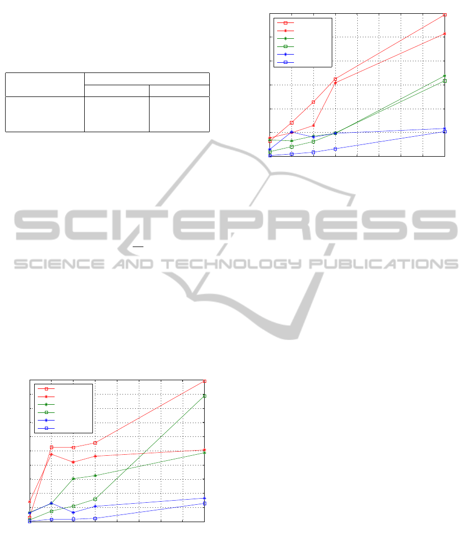
Due to the lower complexity of the suboptimal
SFSD and FPFSD methods, we can to simulate trans-
missions with higher complexity. Figures 3 and 4
have been obtained simulating N
c
= 10000 signals
and varying the number of transmitter antennas (n
T
)
and the constellation sizes.
The speedup results obtained with the parallel
SFSD implementations can be seen in Figure 3, the
value of N
iter
is {2, 4, 6} for QPSK, 16-QAM and 64-
QAM, respectively and L = d
√
n
T
e−1. As we can
see, the multicore version have better performance
than CUDA version when the computational burden
is insufficient to exploit the capabilities of the GPU.
When the number of transmitter antennas n
T
and
constellation size increases, the CUDA implementa-
tion obtain better performance than multicore version.
This is more noticeable from n
T
= 10, since the num-
ber of levels in the FE stage is fixed to L = 3. This
behavior also occurs for the FPFSD detector (see 4).
4 6 8 10 12 14 16 18 20
0
5
10
15
20
25
30
35
40
45
50
n
T
Speedup
64QAM(gpu)
64QAM(omp)
16QAM(omp)
16QAM(gpu)
QPSK(omp)
QPSK(gpu)
Figure 3: Speedup for the SFSD detector with different
constellations and number of transmitter antennas.
4 6 8 10 12 14 16 18 20
0
5
10
15
20
25
30
n
T
Speedup
64QAM(gpu)
64QAM(omp)
16QAM(omp)
16QAM(gpu)
QPSK(omp)
QPSK(gpu)
Figure 4: Speedup for the FPFSD detector with different
constellations and number of transmitter antennas.
6 CONCLUSIONS
This paper presents a set of Soft-Output detectors in-
cluded in the future library for MIMO communica-
tions systems, called MIMOPack, which aims to pro-
vide a set of routines needed to perform the most com-
plex stages in the current wireless communications.
The efficiency of these detectors have been evalu-
ated by comparing the execution time with differ-
ent platform configurations. The variety of detectors
with mixed complexities and performances allows to
cover multiple use cases with different channel con-
ditions and scenarios such as massive MIMO. More-
over, parallel implementations allow the execution of
large simulations over different architectures thus ex-
ploiting the capacity of the modern machines. Re-
sults obtained with the efficient soft-output detectors
presented in this paper demonstrate that MIMOPack
library may become in a very useful tool for compa-
nies involved in the development of new wireless and
broadband standards, which need to obtain results and
statistics of its proposals quickly and also for other re-
searchers making easier the implementation of scien-
tific codes.
ACKNOWLEDGEMENTS
This work has been supported by SP20120646
project of Universitat Polit
`
ecnica de Val
`
encia, by
ISIC/2012/006 and PROMETEO FASE II 2014/003
projects of Generalitat Valenciana; and has been sup-
ported by European Union ERDF and Spanish Gov-
ernment through TEC2012-38142-C04-01.
EfficientSoft-outputDetectors-Multi-coreandGPUimplementationsinMIMOPackLibrary
343

REFERENCES
Barbero, L. G., Ratnarajah, T., and Cowan, C. (2008).
A low-complexity soft-MIMO detector based on the
fixed-complexity sphere decoder. In IEEE Interna-
tional Conference on Acoustics, Speech and Signal
Processing.
Barbero, L. G. and Thompson, J. S. (2008). Fixing the
complexity of the sphere decoder for MIMO detec-
tion. IEEE Transactions on Wireless Communica-
tions, 7(6):2131–2142.
Berenguer, I. and Wang, X. (2003). Space-time coding and
signal processing for mimo communications. Journal
of Computer Science and Technology, 18(6):689–702.
Caire, G., Taricco, G., and Biglieri, E. (1998). Bit-
interleaved coded modulation. IEEE Trans. Inform.
Theory, 44(3):927–946.
Falcao, G., Silva, V., and Sousa, L. (2009). How GPUs
can outperform ASICs for fast LDPC decoding. In In-
ternational Conference on Supercomputing, Yorktown
Heights, New York (USA).
Flynn, M. (1972). Some computer organizations and
their effectiveness. IEEE Transactions on Computers,
21:948–960.
Jalden, J., Barbero, L., Ottersten, B., and Thompson, J.
(2009). The error probability of the fixed-complexity
sphere decoder. IEEE Transactions on Signal Process-
ing, 57:2711–2720.
Kim, J., Hyeon, S., and Choi, S. (2010). Implementation
of an sdr system using graphics processing unit. IEEE
Commun. Mag., 48(3):156–162.
Muller-Weinfurtner, S. (2002). Coding approaches for mul-
tiple antenna transmission in fast fading and ofdm.
IEEE Transactions on Signal Processing, 50:2442–
2450.
NVIDIA (2014). Nvidia programming guide, version 6.0.
http://docs.nvidia.com/.
OpenMP (2013). Application program interface v4.0.
http://www.openmp.org/.
Paulraj, A. J., Gore, D. A., Nabar, R., and Bolcskei, H.
(2004). An overview of MIMO communications - a
key to Gigabit wireless. In Proceedings of the IEEE,
volume 92, pages 198–218.
Roger, S., Ramiro, C., Gonzalez, A., Almenar, V., and Vi-
dal, A. M. (2012). Fully parallel gpu implementa-
tion of a fixed-complexity soft-output mimo detec-
tor. IEEE Transactions on Vehicular Technology,
61(8):3796–3800.
Rusek, F., Persson, D., Lau, B., Larsson, E., Marzetta, T.,
Edfors, O., and Tufvesso, F. (2013). Scaling up mimo:
Opportunities and challenges with very large arrays.
IEEE Signal Processing Magazine, 30(1):40–60.
Wu, M., Sun, Y., Gupta, S., and Cavallaro, J. (2010). Im-
plementation of a high throughput soft MIMO detec-
tor on GPU. Journal of Signal Processing Systems,
64:123–136.
PECCS2015-5thInternationalConferenceonPervasiveandEmbeddedComputingandCommunicationSystems
344
