
A Hybrid Memory Data Cube Approach for High Dimension
Relations
Rodrigo Rocha Silva
1
, Celso Massaki Hirata
1
and Joubert de Castro Lima
2
1
Electronic Engineering and Computer Science Division, Department of Computer Science,
Aeronautics Institute of Technology, São José dos Campos, Brazil
2
Department of Computer Science, Federal University of Ouro Preto, Ouro Preto, Brazil
Keywords: OLAP, Data Cube, Inverted Index, High Dimension, and External Memory.
Abstract: Approaches based on inverted indexes, such as Frag-Cubing, are considered efficient in terms of runtime
and main memory usage for high dimension cube computation and query. These approaches do not compute
all aggregations a priori. They index information about occurrences of attributes in a manner that it is time
efficient to answer multidimensional queries. As any other main memory based cube solution, Frag-Cubing
is limited to main memory available, thus if the size of the cube exceeds main memory capacity, external
memory is required. The challenge of using external memory is to define criteria to select which fragments
of the cube should be in main memory. In this paper, we implement and test an approach that is an
extension of Frag-Cubing, named H-Frag, which selects fragments of the cube, according to attribute
frequencies and dimension cardinalities, to be stored in main memory. In our experiment, H-Frag
outperforms Frag-Cubing in both query response time and main memory usage. A massive cube with 60
dimensions and 10
9
tuples was computed by H-Frag sequentially using 110 GB of RAM and 286 GB of
external memory, taking 64 hours. This data cube answers complex queries in less than 40 seconds. Frag-
Cubing could not compute such a cube in the same machine.
1 INTRODUCTION
The data cube relational operator (Gray et al., 1997)
pre-computes and stores multidimensional
aggregations, enabling users to perform
multidimensional analysis on the fly. A data cube
has exponential storage and runtime complexity
according to a linear dimension increase. It is a
generalization of the group-by relational operator
over all possible combinations of dimensions with
various granularity aggregates (Han, 2011). Each
group-by, called a cuboid or view, corresponds to a
set of cells described as tuples over the cuboid
dimensions.
There are two types of cells in data cubes: base
and aggregate cells. Suppose there is data cube with
3 dimensions. Let us consider a tuple t
1
=(A
1
, B
1
, C
1,
m) of a relation, where A
1
,B
1
andC
1
are dimension
attributes, and m is a numerical value representing a
measure of t
1
. Given t
1,
in our example, a data cube
has seven tuples representing all possible t
1
aggregations, and they are: t
2
=(A
1
,B
1
,*,m),t
2
=(A
1
,
*,C
1
,m),t
4
=(*,B
1
,C
1,
m),t
5
=(A
1
,*,*,m),t
6
=(*,B
1
,*,
m), t
7
=(*, *, C
1
, m), t
8
=(*, *, *, m), where “*” is a
wildcard representing all values of a cube
dimension. Generally speaking, a cube, computed
from relation ABC with cardinalities C
A
, C
B
and C
C
,
can have 2
3
or (C
A
+1)x(C
B
+1)x(C
C
+1) tuples. Our
cube has three dimensions with equal cardinality C
A
=C
B
=C
C
=1.
The dimension increase also makes cube
combinatorial problem harder. If instead of relation
ABC, we consider relation ABCD and C
A
=C
B
=C
C
=
C
D
= 2, we can have 16 tuples of type ABCD, 81
tuples in a full data cube. Most of cube approaches
are not designed for high dimension data cubes.
Frag-Cubing (Li et al., 2004) is the first efficient
high dimension data cube solution. Frag-Cubing
implements an inverted index of tuples, i.e., each
attribute value of a tuple may be associated with n
tuples identifiers. Point queries with two or more
attributes are answered by intersecting tuple
identifiers from attribute values. Frag-Cubing only
implements Equal and Sub-cube query operators.
Frag-Cubing is a main memory based approach, so
huge high dimension data cubes, which require more
139
Silva R., Hirata C. and Lima J..
A Hybrid Memory Data Cube Approach for High Dimension Relations.
DOI: 10.5220/0005371601390149
In Proceedings of the 17th International Conference on Enterprise Information Systems (ICEIS-2015), pages 139-149
ISBN: 978-989-758-096-3
Copyright
c
2015 SCITEPRESS (Science and Technology Publications, Lda.)

main memory than it is available in the machine,
cannot be addressed efficiently. The usage of virtual
memory is managed by the operating system, which
does not take into account all data cube properties.
The result after operating system intervention is an
unacceptable runtime, as our experiments
demonstrate.
In this paper, we implement and test an approach
that is an extension of Frag-Cubing, named H-Frag,
which implements indexing strategies for high
dimension data cubes using a hybrid memory
system. The H-Frag approach selects fragments of
the cube to be stored in main memory and fragments
to be in external memory. The frequencies of
attributes and cardinalities of dimensions are used to
select the memory type for each attribute of a base
relation. Most frequent attributes are stored in main
memory and attribute values with low frequencies
are stored in external memories. Furthermore, H-
Frag avoids operating system interventions - no
operating system swaps are required during H-Frag
cube computation and updates. H-Frag implements
its own swap strategy to load as few information as
possible.
H-Frag enables indexing and querying high
dimension data cubes with billions of tuples. H-Frag
outperforms Frag-Cubing in both query response
time and main memory usage. H-Frag is also a range
cube approach, where query operators greater than,
less than, between, similar, some, distinct, and
different are implemented.
The rest of the paper is organized as follows:
Section 2 details Frag-Cubing, as well as some
promising range query approaches, pointing out their
benefits and limitations. Section 3 details H-Frag
approach, i.e., its architecture and algorithms.
Section 4 describes the H-Frag experiments and
results. Finally, in Section 5, we conclude our work
and point out future improvements of H-Frag.
2 RELATED WORK
There are several cube approaches, but only three of
them implement a sequential high dimension data
cube solution. Frag-Cubing (Li et al., 2004), qCube
(Silva et al. 2013) and Fangling et al(2006)
implement a partial cube approach using inverted
index and bitmap index. There is a clear saturation
curve when full, iceberg, dwarf, multidimensional
cyclic graph (MCG), closed, or quotient approaches
(Brahmi et al., 2012; Ruggieri et al., 2010; Lima and
Hirata, 2011; Xin et al., 2006; Sismanis et al., 2002)
are used for cubes with high number of dimensions.
A high dimension data cube can have 20, 100 or
1000 dimensions and each dimension several
attributes organized as several hierarchies.
Frag-cubing implements the inverted tuple
concept. Each tuple iT has an attribute value, a TID
list, and a corresponding set of measures. For
instance, we consider four tuples: t
1
= (tid
1
, a
1
, b
2
, c
2
,
m
1
), t
2
= (tid
2
, a
1
, b
3
, c
3
, m
2
), t
3
= (tid
3
, a
1
, b
4
, c
4
, m
3
),
and t
4
= (tid
4
, a
1
, b
4
, c
1
, m
4
). These four tuples
produce eight inverted tuples: iTa
1
, iTb
2
, iTb
3
, iTb
4
,
iTc
1
, iTc
2
, iTc
3,
and iTc
4
. For each attribute value, we
build an occurrences list; i.e., for a
1
we have iTa
1
=
(a
1
, tid
1
, tid
2
, tid
3
, tid
4
, m
1
, m
2
, m
3
, m
4
), where the
attribute value a
1
is associated with tuple identifiers
tid
1
, tid
2
, tid
3,
and tid
4
. Tuple identifier tid
1
has
measure value m
1
, tid
2
has measure value m
2
, tid
3
has
measure value m
3,
and tid
4
has measure value m
4
.
Query q = (a
1
, b
4
, COUNT) can be answered by
iTa
1
∩iTb
4
= (a
1
b
4
, tid
3
, tid
4
, COUNT(m
3
, m
4
)). In q,
iTa
1
∩iTb
4
denotes the common tuple identifiers in
iTa
1
and iTb
4
.
The intersection complexity is proportional to the
number of occurrences of an attribute value; more
precisely, it is equal to the size of the smallest list. In
our example, iTb
4
with two tuple identifiers is the
smallest list; therefore, iTb
4
∩iTa
1
is more efficient
than iTa
1
∩iTb
4
. The number of tuple identifiers
associated with each attribute value can be large;
therefore, relations with low cardinality dimensions
and a high number of tuples require high processing
capacity. As TID lists become smaller, the frag-
cubing query becomes faster; consequently, relations
with low skew and both high cardinalities and
dimensions are more suitable to frag-cubing
computation.
qCube (Silva et al., 2013) uses inverted indices
to address a solution to range queries over high
dimension data cubes. Range queries include greater
than, less than, between, similar, some, distinct, and
different query operators to collect several
aggregations and not only a point-unique
summarized result from the data cube. qCube is
main memory based, so some cubes cannot fit in
main memory, requiring operating system swaps that
are always inefficient. In general, as the number of
high dimension tuples becomes higher, hybrid
memory based solutions are required.
3 H-Frag APPROACH
Data input for cube computation in the H-Frag
approach is d-dimensional relation R with n tuples,
where n ⊂ 1, ∞. Formally, R is a set of tuples,
ICEIS2015-17thInternationalConferenceonEnterpriseInformationSystems
140
where each tuple t is defined as t = (tid, D
1
, D
2
, ...,
D
z
). In t, tid attribute is a unique identifier therefore,
in a relation there are no equal tuples, as proposed
by Codd (1972). The number of dimensions is
represented by z, D is a specific dimension, defined
as D
i
= (att
1
, att
2
, … , att
n
) and att is a possible
attribute value of dimension D
i
.
H-Frag architecture has three main components:
computation, query and measure computation.
First, the computation component scans R
completely in order to obtain the frequency of each
attribute value of each R dimension.
Then, the average frequency is calculated, and
the attribute values with frequencies lower than the
average are marked in order to be stored in the
external memory.
R is scanned by the computation component a
second time to select the attribute values to be stored
in external memory. Each attribute value and its list
of tuple identifiers (tids) are stored in external
memory, i.e., a single attribute value can have
several complementary tid‐list in external memory,
since RAM can get full. To avoid that, H-Frag
partitions R into complementary portions defined by
the user, with several tuples each portion.
Each portion can be stored fully in the main
memory. However, in order to avoid attribute values
in the external memory with low number of tids, H-
Frag defines an occurrence percentage for each
attribute value inside a portion. Each attribute value
has to be associated to, at least, 50% of the number
of the tuples in a portion to be stored. When the
frequency of each attribute value reaches the 50% of
the number of the tuples in a portion, the tid‐list of
attribute value is stored in external memory.
The measure values are grouped by portions:
each group of measure values is identified by a tid
interval or range (e.g., in a portion where tuples have
been processed from 1 to 10 the identification of the
file will contain 1_10). This way, H-Frag generates
few files.
However, if the frequencies of attribute values
have not reached 50% of the number of the tuples in
a portion, but if 80% of the available working
memory is being used, all tid-list of processed
attribute values and all measure values are stored in
external memory. H-Frag eliminates the problem
when there are many attribute values below 50% of
a portion, which can happen in relations with high
cardinality and low skew. At the end of each portion,
if an attribute value has not reached 50% of the
current portion and 80% of available working
memory is being not used, it remains in the main
memory and a new portion is loaded to be
processed. Frequent attribute values will demand
several complementary tid-lists stored in external
memory and all of them must be swapped into main
memory to answer a query containing such attribute
values.
Finally, R is scanned for a third time, generating
as an output a map with the top frequent attribute
values of R and their tid‐list. Such a map is
maintained in main memory.
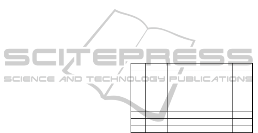
Table 1 illustrates an example where there are
dimensions A, B and C: dimension A has cardinality
3 and the values set {a
1
,a
2
,a
3
}, the dimension B has
the cardinality 3 and the values set {b
1
,b
2
,b
3
}, and
the dimension C has cardinality 2 with {c
1
,c
2
} as the
values set. Table 1 also presents two measures (M1,
M2). The unique identifiers of each tuple are
represented by tids.
Table 1: Input Relation R.
tid A B C M1 M2
1
a
1
b
1
c
1
1.5 1
2
a
2
b
2
c
2
2.5 1
3
a
2
b
2
c
2
2 3
4
a
3
b
3
c
2
78.5 2
5
a
1
b
1
c
1
100 5
6
a
2
b
1
c
2
102.5 4
7
a
3
b
1
c
1
100 2
8
a
1
b
3
c
2
22.5 3
9
a
1
b
3
c
2
13.89 8
First, the frequencies of the attribute values of
each dimension are computed and the result is:
fa
1
=4,f‐a
2
=3,fa
3
=2,fb
1
=4,fb
2
=2,fb
3
=3,fc
1
=3and
fc
2
=6. The attributes to be stored in the external
memory are with the frequency lower than the
average of those attribute value frequency of such
dimension, therefore 3 is the average frequency in
the dimensions A and B, as both dimensions have
three attribute values each one and the total of tuples
in the base is 9. In dimension C, the average
frequency is 4.5 (let´s consider 4). Herewith, the
attributes a
3
,b
2
,b
3
andc
1
are marked to be stored in
the external memory.
R is scanned for the second time in order to store
in the external memory the infrequent attribute
values previously identified. We define R partitioned
into three portions with three tuples each. When
each tid‐list reaches 50% of each portion, this list is
stored in the external memory. After all portions are
scanned, the remaining infrequent attribute values
are stored. Table 2 shows the structure of tid‐list
indexed by its respective attribute values stored in
the main memory.
AHybridMemoryDataCubeApproachforHighDimensionRelations
141
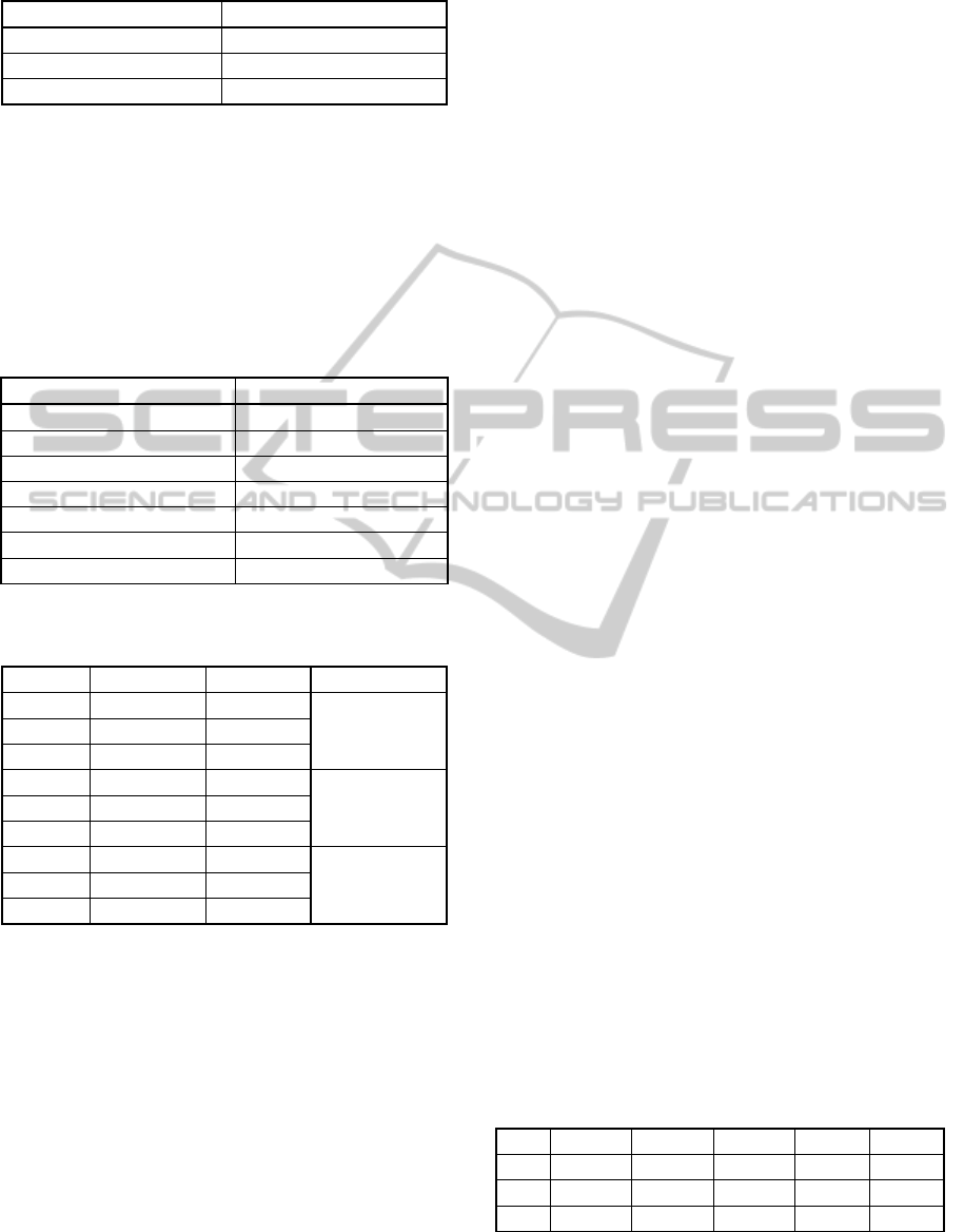
Table 2: Frequent Attribute Values in Primary Memory.
AttributeValue tids
a
1
1,5,8,9
b
1
1,5,6,7
c
2
2,3,4,6,8,9
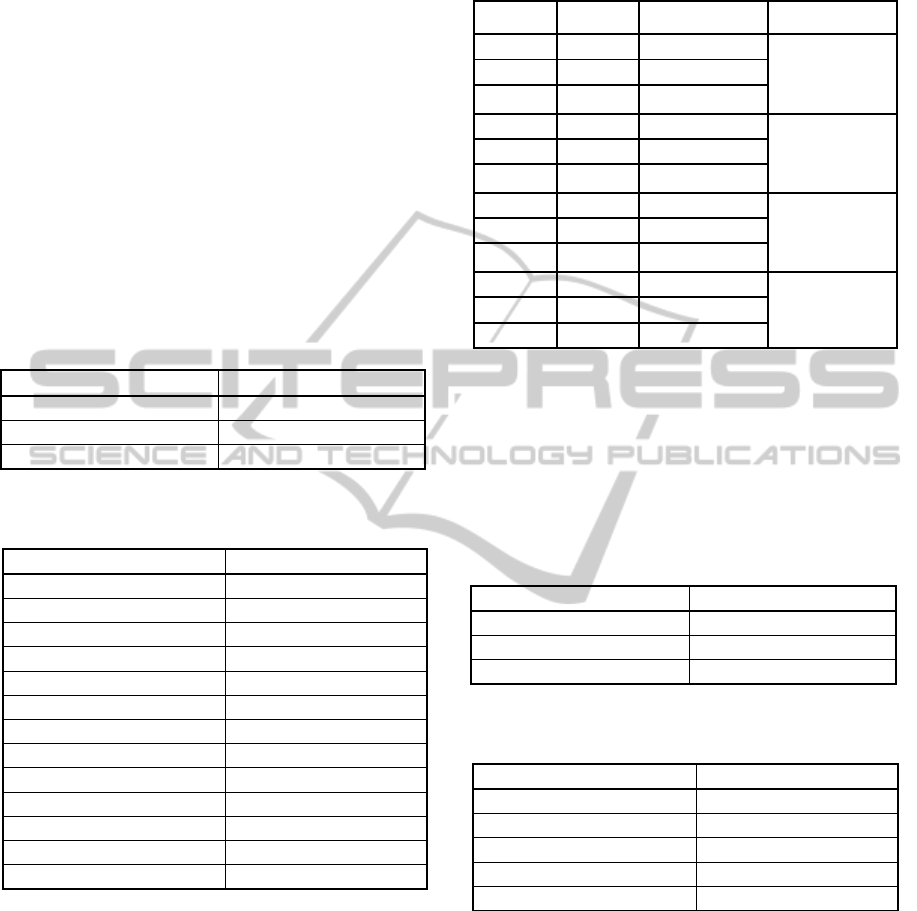
Table 3 illustrates the list structure indexed by its
respective attribute values stored in the external
memory (each line represents a file stored in
external memory). Table 4 presents the cube
measure values with the inverted tuples stored in the
external memory. For each group of measure, a file
is created with the value from all the associated
measures with all the tuples processed in the portion.
Table 3: Attribute Values in External Memory.
AttributeValue Tids
a
2
2,3
a
2
6
a
3
4,7
b
2
2,3
b
3
4,8
b
3
9
c
1
1,5,7
Table 4: Measure Values Relation in External Memory.
Assuming that tuples have been processed every three.
Tids M1 M2 Group
1 1.5 1
1_3
2 2.5 1
3 2 3
4 78.5 2
4_65 100 5
6 102.5 4
7 100 2
7_9
8 22.5 3
9 13.89 8
When the user executes a query, the query
component performs intersections and unions with
tid‐list in the main memory. After obtaining the tid‐
list from the portion of the query that has the
frequent attribute values, the attribute values from
the query that are stored in the portions of the
external memory are processed. The tid‐list obtained
from the query is used to obtain the numerical
measure values, thereby enabling statistical
functions, such as avg, sum, variance and others, to
be calculated by the measure computation
component.
3.1 Computation Algorithm
The computation algorithm has as input a R with set
of tuples t is defined as t= (tid,D1, D2, ..., Dn) and
as output an H-Frag data cube.
Initially, the computation algorithm calculates
the frequency of all attribute values for each R
dimension. These frequencies are stored in an
attsInDisc variable.
After that, the algorithm calculates the average
frequency for each dimension and stores the attribute
values whose frequency is higher than the average in
a variable attsInDisc. This variable indicates the
attribute values that are stored in the external
memory.
For each portion of R, it is verified if each
attribute value frequency is equal to 50% of the
portion dimension frequency and if the 80% of
available working memory is not being used. In this
case, only the attribute value is stored in the external
memory with its tid-list. However, if 80% of
available working memory is being used, all the
attribute values and the group of measure values are
stored in the external memory with its tid-list.
For each portion of R, the attribute values that
even are not stored and the group of measure values
are stored in the external memory.
Finally, we store the set of inverted tuples of the
attribute values not marked to be stored in the
external memory in the main memory.
3.2 Update Algorithm
The inverted index idea is a convenient strategy for
updates where a new tuple is added to R, R attribute
values are merged, new dimensions and new
measures are added to R and dimension hierarchies
are rearranged.
The computation algorithm is used with no
changes in update of a new tuple is added to R.
Example 1: We add three new tuples where one
tuple have new attribute values, a second tuple has
attribute values that are stored in external memory
and a third tuple has attribute values stored in main
memory, as illustrated by Table 5.
Table 5: Update Relation: New Tuples.
tid A B C M1 M2
10
a
4
b
4
c
4
3 7
11
a
3
b
3
c
1
4.7 12
12
a
1
b
1
c
2
5.5 6
The update relation with three new tuples is
ICEIS2015-17thInternationalConferenceonEnterpriseInformationSystems
142
scanned. For all attribute value of each tuple, H-Frag
verifies if it has already been computed. If it was
computed, it is verified where it is stored: main or
external memory. In case the attribute value has
been stored in main memory and there is main
memory available, the attribute value with tid-list is
stored in main memory. If there is no main memory
available, the attribute value with tid-list is stored in
external memory. In case the attribute value was
stored in external memory the tid-list is stored in
external memory. In case there is no working
memory for update, the attribute values stored in
main memory are discarded.
The H- Frag data cube update after insertion of
three new tuples is illustrated in Tables 5, 6, 7 and 8.
Table 6: Frequent Attribute Values in Main Memory After
Example update 1.
AttributeValue tids
a
1
1,5,8,9,12
b
1
1,5,6,7,12
c
2
2,3,4,6,8,9,12
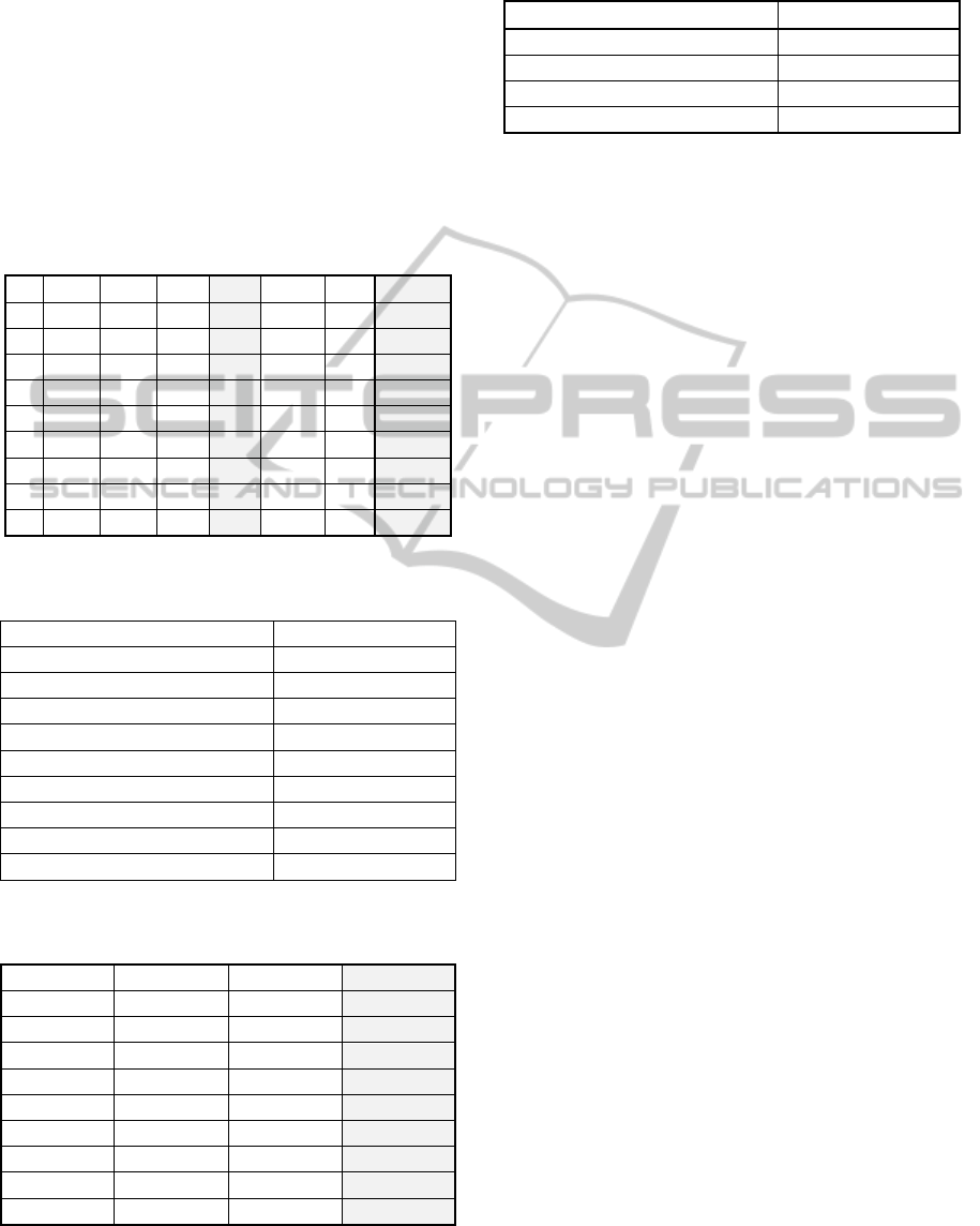
Table 7: Attribute Values in External Memory After
Example update 1.
AttributeValue tids
a
2
2,3
a
2
6
a
3
4,7
a
4
10
a
3
11
b
2
2,3
b
3
4,8
b
3
9
b
3
11
b
4
10
c
1
1,5
c
1
11
C
4
10
Updates where R attributes are merged and these
attribute values are in external memory, each tid-list
must be loaded into main memory to be merged. If
the result generates an attribute more frequent from
the same dimension, this attribute is stored in main
memory after the attribute that has the overcome
frequency be stored in external memory. These
updates, in general, are trivial and its computational
cost depends on the frequency of the attribute in R.
Table 8: Measure Values Relation in External Memory,
After Example update 1.
Tids M1 M2 Group
1 1.5 1
2 2.5 1 1_3
3 2 3
4 78.5 2
5 100 5 4_6
6 102.5 4
7 100 2
8 22.5 3 7_9
9 13.89 8
10 3 1
10_12
11 4.7 12
12 5.5 6
Example 2: Suppose that attribute value a
2
and a
3
are merged as a
9
, the attribute value a
9
will have the
highest frequency and will replace
a
1
attribute value
in main memory. Therefore the attribute value a1
will be stored in external memory, as illustrated by
Tables 9 and 10.
Table 9: Frequent Attribute Values in Main Memory After
Example update 2.
AttributeValue Tids
a
9
2,3,4,6,7
b
1
1,5,6,7
c
2
2,3,4,6,8,9
Table 10: Attribute Values in External Memory After
Example update 1.
AttributeValue Tids
a
1
1,5,8,9
b
2
2,3
b
3
4,8
b
3
9
c
1
1,5,7
Approaches that do not inverted indices or any
other method that fragment the cube to assemble
them efficiently after requiring a complete
reconstruction of the data cube, something extremely
costly in small bases of a midsize, however
impracticable to massive bases.
Updates where new dimensions and measures
can be added to R require the new dimension or
measure be traversed, so their attribute values are
associated with tids of the computed cube.
Example 3: The Tables 11, 12, 13 and 14
illustrate the result of updates, where new dimension
AHybridMemoryDataCubeApproachforHighDimensionRelations
143
D and new measure M3 are added to R. A complete
scan of new dimensions and measures are
mandatory. A dimension D and a new measure M3
are added to R, but H-Frag does not require
recalculations. Thus only the new attribute values
and measure values are inserted with the respective
tid‐list, according to the Tables 11, 12, 13 and 14.
Updates whose dimension hierarchies are
rearranged do not impact the data cube computed by
H-Frag, since a query can be proceed in any order.
Table 11: Update Relation: new dimension D and new
measure M3.
tid A B C D M1 M2 M3
1
a
1
b
1
c
1
d
1
1.5 1 6
2
a
2
b
2
c
2
d
1
2.5 1 5.66
3
a
2
b
2
c
2
d
1
2 3 78.98
4
a
3
b
3
c
2
d
1
78.5 2 2.98
5
a
1
b
1
c
1
d
3
100 5 1.65
6
a
2
b
1
c
2
d
2
102.5 4 2.69
7
a
3
b
1
c
1
d
1
100 2 6.87
8
a
1
b
3
c
2
d
3
22.5 3 98.999
9
a
1
b
3
c
2
d
2
13.89 8 78.995
Table 12: Attribute Values in External Memory After
Example update 3.
AttributeValue tids
a
2
2,3
a
2
6
a
3
4,7
b
2
2,3
b
3
4,8
b
3
9
c
1
1,5,7
d
2
6,9
d
3
5,8
Table 13: Measure Values Relation in External Memory:
After Example update 3.
tids M1 M2 M3
1 1.5 1 6
2 2.5 1 5.66
3 2 3 78.98
4 78.5 2 2.98
5 100 5 1.65
6 102.5 4 2.69
7 100 2 6.87
8 22.5 3 98.999
9 13.89 8 78.995
Table 14: Frequent Attribute Values in Main Memory.
After Example update 3.
AttributeValue tids
a
1
1,5,8,9
b
1
1,5,6,7
c
2
2,3,4,6,8,9
d
1
1,2,3,4,7
3.3 Query Algorithm
A Data cube H-Frag can answer queries of type Q,
generating as output three or more sub-lists of tids,
derived from two possible sub-types of queries:
point queries and queries with multiple
summarizations. A point query is performed when
using a filter with equality operator, queries that
have as a result multiple aggregations are those
where range filters or inquire filters are used. Filters
with different operators may be used in Q, each filter
applied to one dimension or measure of R. Thus,
three possible sub-queries are generated from Q: pQ
(queries with equality filters), rQ (queries with range
filters) and iQ (queries with inquire filters). A single
result Q consolidates the results of the three possible
sub-queries with an intersection algorithm
with complexity O(n), where n is the number of
elements in the set.
A point query pQ ∈ Q. For pQqueries we have
as a result a unique aggregation of a set of attributes
of R. rQ ∈ Q represents range queries in different
dimensions. A query rQ may have as result a set of
summarizations from attributes present in R. An
inquire sub-query iQ has as a result the combination
of dimensions cardinalities. iQ ∈ Q, represents
inquire, where a set of operators iOp (subcube +
distinct) are defined for different dimensions. The
range operator rQ is defined as rOp=(greaterthan
+lessthan+
between+some+different+similarx
(v
1
,v
2,
…,v
n
)). The symbol '+' represents the logical
operator OR and 'x' represents the logical operator
AND. The values defined by the user for a range
operator are represented by (v
1
,v
2,
…,v
n
).
A sub-query inquire iQ has as a result a set of
combinatory aggregations of different dimensions.
iQ ∈ Q, represents query inquire where a set of
operators iOp (subcube + distinct) are defined to
different dimensions. A subcube of a dimension is
composed by every possible aggregations of a
dimension, including the wildcard all (*).
When operators rQ or iQ are used as filters in a
dimension, we have a query of a subcube to this
dimension. The result is composed by every possible
aggregations of this dimension including *. To each
ICEIS2015-17thInternationalConferenceonEnterpriseInformationSystems
144

attribute value of dimension i, there is a tid‐list.
Thus, the tid‐list of (pQ∩rQ) are intersected with
each tid‐list of the dimension i. The result of the
intersection is the tid‐list obtained from the query.
There are
∏
Ci 1
results, then Q has SC
subcube operators, Ci indicates the dimension i
cardinality and SC is the number of subcube filters.
The operators subcube and distinct are identical
to one dimension. For two or more dimensions the
number of distinct aggregations will be
∏
intersections with tids of (pQ∩rQ), so it is
also a costly computational processing. In the
approach H-Frag the sub-query of Q are reorganized
in order to optimize the processing performance.
From a cube H-Frag, a filter F is executed in a
query pQ. Being F defined as F:{op
1
∩op
2
∩... ∩
op
n
}, where op
i
is the operator i
th
EQUAL of F
applied to dimension i of H-Frag. In a query rQ from
a data cube, H-Frag executes a filter F´. This way,
tids of pQ are intersected with tids of rQ. The
definition of F´ is given by F´:{µ
1
∩µ
2
∩...∩µ
n
},
where µ
i
is the operator i
th
RANGE of F´ applied to
dimension i of H-Frag. F and F´ are filters applied to
different dimensions. Each µ
i
returns a tid‐list for
the values that meet the criteria defined by an
operator rOp. Thus, a group of intersection of the
tid‐list is executed for each possible association
among attributes instantiated in each sub-query and
these intersections are always initiated from the
attributes with the smallest tid‐list.
Queries iQ are also combinatorial, therefore a
query iQ inquire receives a data cube H‐Frag, and
executes a third filter F ´´. The tids of iQ are
intersected with tids resulting from (pQ∩rQ). Filter
F´´ is defined as F´´: {Ƭ
1
∩ Ƭ
2
∩ ... ∩ Ƭ
n
}, where Ƭ
i
is the operator i
th
INQUIRE of F ´´ applied to
dimension i of H-Frag. F, F´e F´´ are filters applied
to different dimensions.
The first sub-queries executed are always the
point queries. Then, the range and inquire Q queries
are executed. At each sub-query the tid‐list is
retrieved. When attributes are in main memory, that
is, when these are frequent attributes in the
dimension, this set is retrieved in a single access.
When the attributes have lower frequency in the
dimension, their tid‐list are retrieved from external
memory. In this case, since this set can be
fragmented into several portions in external
memory, there are numerous costly readings. To
reduce the cost of intersections, the last fragment is
loaded first in main memory, since it may have a
few tuples, consequently a smaller tid‐list and lower
cost of intersection with subsequent fragments of a
certain attribute of R.
Example 4: Suppose a user submits a query
q={?,?,c
2
}. H-Frag first fetches the tid-list of the
instantiated dimension by looking at cell (c
2
). This
returns (c
2
):{1,5,4,6,8,9}. See that if there
were no inquired dimensions in the query, we would
finish the query here and return 6 as the final count.
Next, H-Frag fetches the tid-lists of the inquired
dimensions: A and B. These are
{(a
1
:{1,5,8,9})}, {(a
2
:{2,3,6})},
{(a
3
:{4,7})}, {(b
1
:{1,5,6,7})},
{(b
2
:{2,3})} and {(b
3
:{4,8,9})}.
Intersect among them and with the instantiated
c
2
and we get {(a
1
c
2
:{8, 9}), (a
2
c
2
:{2,
3,6}), (a
3
c
2
:{4}), (b
1
c
2
:{6}),
(b
2
c
2
:{2,3}) and (b
3
c
2
:{4,8,9})}. This
corresponds to a base cuboid of six tuples: {(a
1
,
b
1
, c
2
), (a
2
, b
1
, c
2
) , (a
1
, b
2
, c
2
) , (a
1
,
b
2
, c
2
) , (a
1
, b
3
, c
2
) and (a
3
, b
3
, c
2
)}.
Suppose that at some decision-making process it
is necessary do a filter with a range operator.
Example 5: If user submits a query q={a
2
,
>b
1
, c
2
}.
H-Frag first fetches the tid-list of the instantiated
dimensions by looking at cell (a
2
, c
2
). This
returns (a
2
, c
2
):{2,3,6}.
Next, H-Frag fetches the tid-lists of the range
dimension: A. These are {(b
2
:{2,3})} and
{(a
3
:{4,8,9})}. Intersect them with the
instantiated base and we get {(b
2
:{2, 3})}.
This corresponds to a base cuboid of one tuple:
{(a
2
, b
2
, c
2
)}.
The algorithm for point, range and inquire
queries works as follow: initially, for each sub-
query, the tids (lines 4 and 6) associated with the
attributes instantiated in each dimension are
retrieved. In case the attribute value is in external
memory, it is retrieved a fragment at a time starting
with the last one. After the intersection, the lists are
merged (line 5) until intersections with all tidsoccur
in external memory. Next, the intersections occur
among tid‐list of attributes for each possible
summarization. The intersection always starts from
lists with fewer tids (lines 7-12). Finally, all
measures defined in Q are calculated (line 13).
Algorithm 1 (Query) performing point, range,
and inquire queries;
Input: (1) H-Frag data cube and (2) user query
Q;
Output: H-Frag_R, which includes aggregations
processed by the computation algorithm and
completed by the query algorithm.
AHybridMemoryDataCubeApproachforHighDimensionRelations
145
Method:
1. for each sub-query in Q{ //pQ, rQ or iQ
2. for each attribute in D
i
{
3. if attsInDisk contains attribute{
4. attribute.tids recover disk
5. tids ← tids U attribute.tids
}else{
6. tids ← attribute.tids
}
7. for each tid
i
in
tids {
8. if tid
i
∩ [att
1
, …, att
n
]{
9. RQ
i
← tid
i
∩ [att
1
, …, att
n
]
}
10. if tid
i
∩ [att
1
, att
2
, …, att
n
]{
11. IQ
i
← tid
i
∩ [att
1
, …, att
n
]
}
}
}
12. hFqR ← RQ
i
∩ IQ
i
;
}
13. hFqR ← calcMeasures(hFqR,Q,hFragDiM);
4 EXPERIMENTS
Aiming to verify efficiency and scalability of the
proposed approach, a thorough study was conducted.
Experiments with H-Frag and Frag-Cubing
approaches, testing computation algorithms and
queries provided by both approaches, were
conducted. H-Frag algorithms were coded in Java 64
bits (version 8.0). Frag-Cubing is a C++
implementation provided by authors and compiled
for 64 bits (http://illimine.cs.uiuc.edu/). H-Frag
approach has two versions: main memory version
and hybrid version. The hybrid uses both memories.
The main-memory H-Frag version just maintain all
data in main memory, so no conceptual changes
were introduced to implement H-Frag only in RAM.
Query response times using hybrid H-Fragapproach
considers both external and main memories accesses
times. None of the experiments using H-Frag
exceeded the physical limit of the machine main
memory, so approaches did not require Operating
Systems swaps.
The algorithms are sequential versions. The use
of multiprocessor architecture is still useful, since
there is implicit parallelism. We ran the algorithms
on two processors: six-core Intel Xeon with 2,4 GHz
each core, cache of 12 MB and 128 GB of RAM
DDR3 1333MHz. The disk is SAS 15k rpm with
64MB of cache. The operating system is Windows
HPC (High Performance Computing) Server 2008
version of 64 bits. All experiments were executed
five times and we removed the longest and shortest
runtimes, calculating the average of the three
remaining runtimes.
4.1 Computing Different Numbers of
Tuples
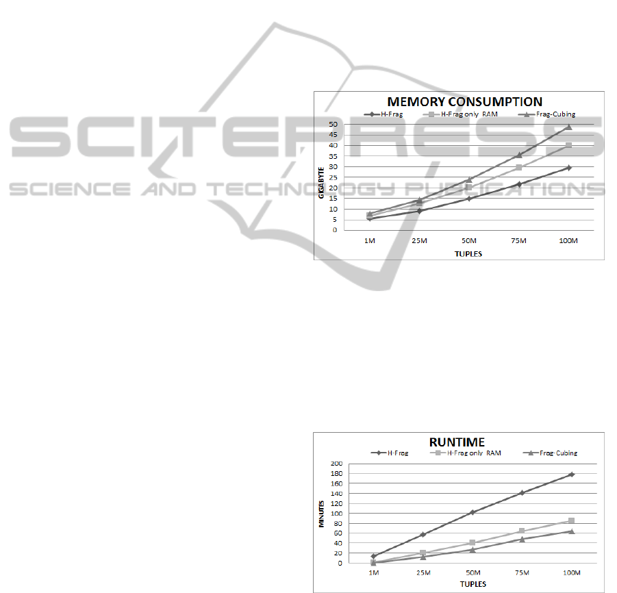
The tests varying the amount of tuples had linearly
stable behaviour in both approaches. We used
relations with T=1M, 25M, 50M, 75M and 100M, D
= 15, C=10
4
e S=0. In general, H-Frag approach had
memory consumption 20 to 35% lower than Frag-
Cubing approach when working only in main
memory, while the hybrid H-Frag consumed 45% to
65% less memory than Frag-Cubing, as Figure 1
illustrates.
Figure 1: H-Frag, H-Frag only main memory and Frag-
Cubing memory consumptions with different tuples:
D=15, S=0, C=10
4
.
The cubes runtimes for the respective relations were
also linear, as it can be observed in Figure 2. In the
worst scenario, H-Frag was three to four times
slower than Frag-cubing when computing a partial
cube; however, this is a reasonable result if we
consider that H-Frag uses external storage.
Figure 2: H-Frag, H-Frag only main memory and Frag-
Cubing runtimes with different tuples: D=15, S=0, C=10
4
.
ICEIS2015-17thInternationalConferenceonEnterpriseInformationSystems
146
4.2 Computing Different Numbers of
Dimensions
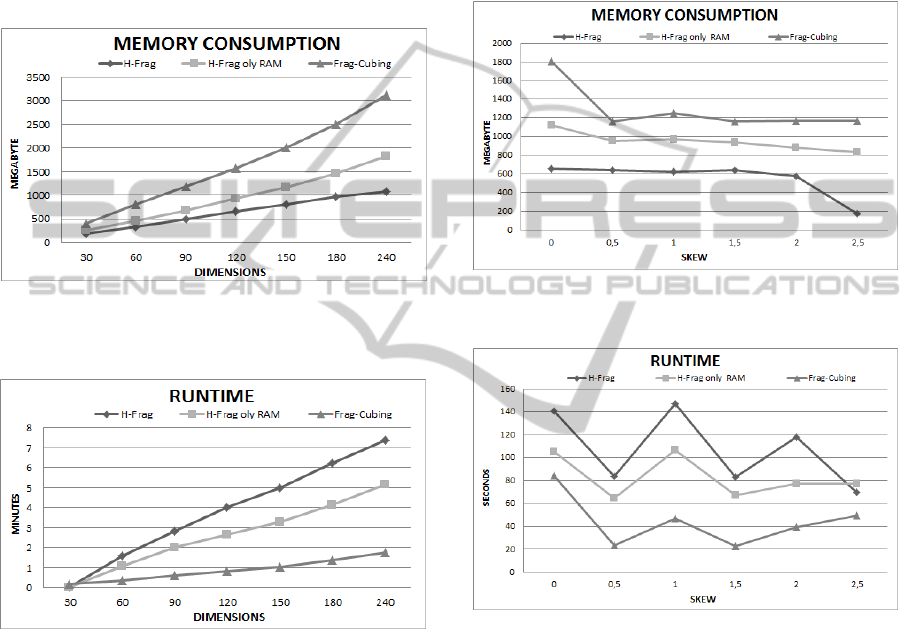
The results of experiments in which the number of
data cube dimensions varied are presented in Figure
3. For these experiments, relations with D = 30, 60,
90, 120, 150, 180 and 240, T = 10 M, and C = 10
4
were used. The memory consumption was linear for
both approaches; however, Frag-Cubing required
35% to 47% more memory.
Figure 3: H-Frag, H-Frag only main memory and Frag-
Cubing memory consumptions with different dimensions:
T = 10
7
, S = 0, and C = 10
4
.
Figure 4: H-Frag, H-Frag only main memory and Frag-
Cubing runtimes with different dimensions: T = 10
7
, S =
0, and C = 10
4
.
The runtimes were also linear, as it can be observed
in Figure 4. In general, H-Frag was between 3.5 and
5 times slower than the Frag-Cubing.
4.3 Computing Skewed Relations
We evaluated data cube computations using base
relations with different skews: S = 0, 0.5, 1, 1.5, 2,
and 2.5, D = 15, T = 10
7
,
and C = 10
4
.
Figure 5 and 6 illustrate memory consumption
and runtime results. In the figure, H-Frag and Frag-
Cubing approaches show the same behavior; i.e., as
skew increased, runtime decreased. However, H-
Frag took 1.6 to 1.3 more times than Frag-Cubing
using only main memory. Skewed base relations are
very common in real scenarios, where few attribute
values are present in almost all tuples. H-Frag stores
frequent attribute values in main memory and
skewed base relations has more frequent attributes
than uniform ones; consequently, H-Frag use more
working memory to compute such relations and
became faster.
Figure 5: H-Frag and Frag-Cubing memory consumptions
with different skews: D = 15, T = 10
7
and C = 10
4
.
Figure 6: H-Frag and Frag-Cubing runtimes with different
skews: D = 15, T = 10
7
and C = 10
4
.
In all scenarios, H-Frag significantly reduced
memory usage in representing a partial cube. It is
evident from the results that Frag-Cubing consumed
23% more main memory than the H-Frag approach
when the base relation was uniform (S = 0);
however, the difference increased as skew increased.
Frag-cubing memory consumption was 50%
higher than that of main memory in base relations
with S = 2.5. In relations skewed, approximately half
of the attribute values were stored in main memory
and half were propagated to external memory. The
significant decrease in memory consumption was
justified by the irregular frequency of attribute
values; therefore, the critical cumulative frequency
could be found in all attribute values. Thus, all tid‐
AHybridMemoryDataCubeApproachforHighDimensionRelations
147
lists were propagated in external memory; only the
references for each tid‐list are stored in main
memory.
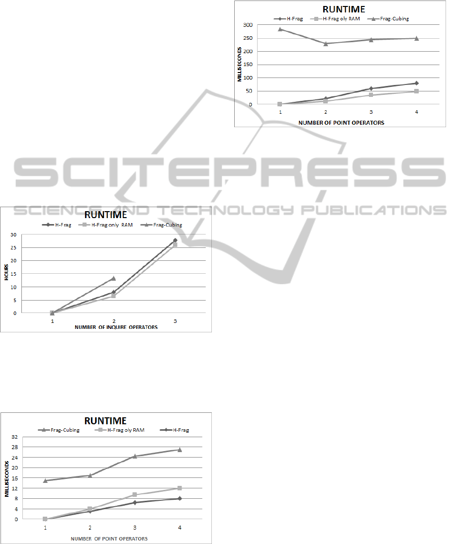
4.4 Query Response Time
Frag-Cubing response times are slower than H-Frag
(about 2-5 times), even in scenarios where there are
many attribute values stored in external memory.
Figure 7 illustrates experiments using the relation R
with T = 10
7
; C = 10
4
; D = 30, S = 0.
Queries with more than two sub-cube operators
cannot be answered by Frag-Cubing, since there is
not enough continuous memory in 128GB of RAM
to allocate many big size arrays with many empty
cells. Frag-Cubing duplicates an array size when it
reaches its limit. In contrast, the number of small
complementary arrays enables H-Frag to produce
huge amount of summarized results. Dimension
rearrangements based on cardinalities also reduce
inquire query response times drastically.
Figure 7: Query Response time with inquire operators: T =
10
7
; C = 10
4
; D = 30, S = 0.
Figure 8 depicts results of experiments with queries
using attribute values higher than the critical
frequency.
Figure 8: Query response time with point operators, using
attribute values higher than the critical frequency: T = 10
7
,
C = 10
4
, D = 30, and S = 0.
Figure 9 illustrates results of experiments with
queries using attribute values lower than the critical
frequency.
Figure 9: Query response time with point operators, using
attribute values lower than the critical frequency: T = 10
7
,
C = 10
4
, D = 30, and S = 0.
4.5 Massive Data Cube
A relation with T = 10
9
tuples was computed by the
H-Frag approach. This experiment took 64 hours
and consumed 126 GB of RAM. The results show
that it is possible to compute massive cubes using
the H-Frag approach with no operating system
swaps, thereby enabling both updates and queries.
Queries with five range operators, ten point
operators, and one inquire operator were answered
in less than 35 seconds. To the best of our
knowledge, there is no other sequential cube
approach that efficiently answers high-dimensional
range queries from relations with T = 10
9
tuples.
Data cubes with a high number of tuples could
not be computed by the Frag-Cubing approach using
just main memory. This was demonstrated by trying
to compute a base relation with 200 million tuples
and 60 dimensions.
5 CONCLUSIONS
To enable the computation of massive data cubes
with massive amount of tuples, we implemented and
tested an approach named H-Frag. This approach is
an extension of Frag-Cubing approach, enabling
hybrid memory capabilities, so data cubes with 10
9
tuples can be indexed. H-Frag uses the following
strategy: attribute values with high frequencies are
stored in main memory and attribute values with low
frequencies are stored in external memory.
The experiments show that H-Frag is an effective
solution for data cubes with high number of tuples.
The results show that H-Frag has linear runtime and
ICEIS2015-17thInternationalConferenceonEnterpriseInformationSystems
148

memory consumption when the number of tuples
increases. Memory consumption of the hybrid
version H-Frag is always lower than Frag-Cubing
approach. When compared with Frag-Cubing, H-
Frag has similar performance in point queries, but
H-Frag approach outperforms Frag-Cubing in
inquire queries, producing answers 9 times faster
than Frag-Cubing approach. H-Frag is designed for
queries types proposed in qCube (Silva et al., 2013),
so H-Frag is also a range cube approach. In the
experiments, we had scenarios where Frag-Cubing
approach failed to index the data cube caused by
lack of main memory. The H-Frag hybrid memory
approach is, on average, 3 times slower than Frag-
Cubing in indexing a cube, which can be also
considered a promising result, since H-Frag uses
external memories to support huge data cubes. A
massive test with 60 dimensions and 10
9
tuples was
conducted to prove that H-Frag is robust and can be
used in extreme scenarios.
There are some improvements to H-Frag
approach. Among them, we can mention computing
and updating experiments for holistic measures,
which are extremely costly and important for
decision making. Top-k multidimensional queries is
part of our interest, since inverted index is also
useful for this type of problem.
ACKNOWLEDGEMENTS
This work was partially supported by ITA, UFOP,
FATEC-MC and by FAPESP under grant No.
2012/04260-4 provided to the authors.
REFERENCES
Brahmi, H., Hamrouni, T., Messaoud, R., and Yahia, S.
“A new concise and exact representation of data
cubes,” Advances in Knowledge Discovery and
Management, Studies in Computational Intelligence
(vol. 398), Springer, Berlin-Heidelberg, 2012, pp. 27–
48.
Codd, E. F. “Relational completeness of data base
sublanguages,” R. Rustin (ed.), Database Systems,
Prentice Hall and IBM Research Report (RJ 987), San
Jose, California, 1972, 65-98.
Gray, J., Chaudhuri, S., Bosworth, A., Layman, A.,
Reichart, D., Venkatrao, M., Pellow, F., and Pira-hesh,
H. “Data cube: a relational aggregation operator
generalizing group-by, cross-tab, and sub-totals,” Data
Mining and Knowledge Discovery (1), 1997, 29–53.
Han, J. Data Mining: Concepts and Techniques. Morgan
Kaufmann Publishers Inc., San Francisco, CA, USA,
2011.
Li, X., Han, J., and Gonzalez, H. “High-dimensional
OLAP: a minimal cubing approach,” Proceedings of
the International Conference on Very Large Data
Bases, 2004, pp. 528–539.
Lima, J. d. C. and Hirata, C. M. “Multidimensional cyclic
graph approach: representing a data cube without
common sub-graphs,” Information Sciences 181 (13),
July 2011, 2626–2655.
Ruggieri, S., Pedreschi, D., and Turini, F. “Dcube:
discrimination discovery in databases,” Proceedings of
ACM SIGMOD International Conference on
Management of Data, New York, NY, USA, 2010, pp.
1127–1130.
Silva, R. R., Lima, J. d. C., and Hirata, C. M. “qCube:
efficient integration of range query operators over a
high dimension data cube,” Journal of Information
and Data Management 4 (3), 2013, 469–482.
Sismanis, Y., Deligiannakis, A., Roussopoulos, N., and
Kotidis, Y. “Dwarf: shrinking the petacube,”
Proceedings of ACM SIGMOD International
Conference on Management of Data, New York, NY,
USA, 2002, pp. 464–475.
Xin, D., Shao, Z., Han, J., and Liu, H. “C-cubing: efficient
computation of closed cubes by aggregation-based
checking,” International Conference on Data
Engineering, Atlanta, Georgia, USA, 2006, pp. 4.
AHybridMemoryDataCubeApproachforHighDimensionRelations
149
