
Dimensionality Reduction for Supervised Learning in
Link Prediction Problems
Antonio Pecli, Bruno Giovanini, Carla C. Pacheco, Carlos Moreira, Fernando Ferreira,
Frederico Tosta, Júlio Tesolin, Marcio Vinicius Dias, Silas Filho, Maria Claudia Cavalcanti
and Ronaldo Goldschmidt
Military Institute of Engineering, Pr. General Tiburcio, 22290-270, Rio de Janeiro, RJ, Brazil
Keywords: Link Prediction, Supervised Learning, Machine Learning, Dimensionality Reduction.
Abstract: In recent years, a considerable amount of attention has been devoted to research on complex networks and
their properties. Collaborative environments, social networks and recommender systems are popular
examples of complex networks that emerged recently and are object of interest in academy and industry.
Many studies model complex networks as graphs and tackle the link prediction problem, one major open
question in network evolution. It consists in predicting the likelihood of an association between two not
interconnected nodes in a graph to appear. One of the approaches to such problem is based on binary
classification supervised learning. Although the curse of dimensionality is a historical obstacle in machine
learning, little effort has been applied to deal with it in the link prediction scenario. So, this paper evaluates
the effects of dimensionality reduction as a preprocessing stage to the binary classifier construction in link
prediction applications. Two dimensionality reduction strategies are experimented: Principal Component
Analysis (PCA) and Forward Feature Selection (FFS). The results of experiments with three different
datasets and four traditional machine learning algorithms show that dimensionality reduction with PCA and
FFS can improve model precision in this kind of problem.
1 INTRODUCTION
For the last years, the constant advances in
information technology have significantly
contributed to increase the amount of interconnected
data around the world. In this scenario, many large,
complex and dynamic digital networks have
emerged. For example, social networks,
collaborative environments and recommender
systems, just to name a few, are complex networks
provided by Web 2.0 and e-Science. Both scientific
and industrial communities have devoted a
considerable amount of attention to the investigation
of such networks and their properties (Liben-Nowell
and Kleinberg, 2003). Many studies model networks
as graphs, where a vertex (node) represents an item
in the network (e. g. person, web page, product,
movie, photo, etc) and an edge represents some sort
of association between the corresponding items (e.g.
a purchase connects the product and the client).
Complex networks are very dynamic, since new
vertices and edges can be added to the graph over
the time. Understanding the reasons that make the
networks evolve is a complex question that has not
been properly answered yet. One major but
comparatively easier problem in the study of
network evolution is the link prediction task. It
consists in predicting the likelihood of an association
between two not interconnected nodes in the graph
to appear (Lü and Zhou, 2011). We have noticed that
link prediction has been applied for two different
tasks: predicting “future” links (Liben-Nowell and
Kleinberg, 2003), when the goal is to discover which
links will appear in the future, and predicting
“missing” links (Lü and Zhou, 2011), used for
inferring links that already exist in the network, but
are not represented yet.
One of the approaches to the link prediction
problem is based on supervised learning (Hasan et
al, 2006; Li and Chen, 2009; Pujari and Kanawati,
2012; Sa and Prudencio, 2011; Benchetarra et al.,
2010). Such approach converts original data to a
binary classification problem. In this problem, each
data point corresponds to a pair of vertices with a
class label denoting their link status: positive if the
association between the two vertices exists,
295
Pecli A., Giovanini B., C. Pacheco C., Moreira C., Ferreira F., Tosta F., Tesolin J., Vinicius Dias M., Filho S., Claudia Cavalcanti M. and Goldschmidt R..
Dimensionality Reduction for Supervised Learning in Link Prediction Problems.
DOI: 10.5220/0005371802950302
In Proceedings of the 17th International Conference on Enterprise Information Systems (ICEIS-2015), pages 295-302
ISBN: 978-989-758-096-3
Copyright
c
2015 SCITEPRESS (Science and Technology Publications, Lda.)

negative, otherwise. Additional features must be
added to the dataset in order to describe its data
points and represent some sort of proximity between
the pair of vertices. A machine learning algorithm is
applied to the enriched dataset in order to generate a
classification model.
Many features have been experimented in
supervised learning for link prediction problems
(Hasan and Zaki, 2011). Typically, these features are
classified in three groups: (a) node and edge
information (e.g. client’s age, job location, etc); (b)
aggregated features (e.g. sum of e-mails, sum of
contacts, etc); (c) topological measures extracted
from the graph (e.g. common neighbors, jaccard’s
coefficient, etc). Choosing which features to add to
the dataset is crucial for the learning process. It is a
typical optimization problem where there is a search
for a reduced set of features that preserves, as much
as possible, the original amount of information
available in the dataset.
Although many works have reported promising
results with the binary classification approach for
link prediction, choosing the set of features to train
the classifiers is acknowledged to be a major
challenge (Hasan and Zaki, 2011).
The machine learning community has developed
many methods to deal with the high-dimensional
space problem (Yu and Liu, 2003; Caruana et al.,
2008). In general, these methods are based on two
approaches (Kohavi and John, 1997): filter and
wrapper. The filter approach consists in calculating
some evaluation metric (such as correlation or
information gain) from the dataset in order to select
the features that lead to better evaluations. On the
other hand, the wrapper approach is iterative and, for
each iteration, selects a subset of features, reduces
the original dataset (using the selected features) and
uses it to construct and evaluate a predictive model.
This process is repeated until a stopping criterion is
satisfied.
Dimensionality reduction techniques can also be
classified in two groups: feature selection and
feature extraction. The main difference between
them is that the first group does not change original
attributes and the second one transforms original
features in new attributes.
Despite its acknowledged importance for
supervised learning tasks, few works have
investigated the effects of dimensionality reduction
in link prediction. Table 1 shows examples of
dimension reduction techniques according to the
classifications presented above.
Feature Selection for Link Prediction – FESLP
(Xu and Rockmore, 2012) and Cross-Temporal Link
Prediction – CTLP (Oyama et al., 2011) have been
specifically designed to be used in link prediction
applications. FESLP selects features based on their
correlation and information gain. CTLP assumes that
features useful for link prediction change over time
and, thus, searches for sets of features which best
describes nodes and theirs variations as time passes
by. Oyama et al., (2011) used CTLP in a dynamic,
time evolving environment to determine the
identities of real entities represented by data objects
observed in different time periods. Xu and
Rockmore (2012) ran their experiments with
datasets generated from an email network of a large
academic university.
Forward Feature Selection – FFS (Freitas, 2002)
and Principal Component Analysis – PCA (Jackson,
1991) are methods traditionally used by the machine
learning community.
FFS is iterative. In each iteration, FFS searches
for a feature that, combined to a set of selected
features, builds a reduced dataset that leads to the
best predictive model (according to some criterion,
such as precision or recall, for example). Its loop
will perform until no predictive model built in the
current iteration shows improvement. Initially, the
set of selected features is empty and FFS builds as
many reduced datasets as the number of attributes in
the original dataset (each reduced dataset contains
exactly one attribute plus the class, target of the
problem).
PCA is a statistical technique that uses an
orthogonal transformation to convert a dataset of
possibly correlated features into a set of linearly
uncorrelated attributes called principal components.
The number of principal components is less than or
equal to the number of original features. Such
components are orthogonal because they are the
eigenvectors of the covariance matrix, calculated
with the attributes of the original dataset.
To the best of our knowledge, both FFS and PCA
have never been used to reduce dimension in link
prediction applications.
Table 1: Examples of Dimensionality Reduction Methods.
Methods Approach Feature Treatment
FESLP Filter Selection
CTLP Filter Selection
PCA Filter Extraction
FFS Wrapper Selection
So, this paper evaluates the effects of PCA and
FFS as dimensionality reduction preprocessing
techniques to the binary classifier construction in
link prediction applications. In constrast to FESLP
and CTLP, we have run our experiments over three
ICEIS2015-17thInternationalConferenceonEnterpriseInformationSystems
296

open and popular datasets (DBLP, Amazon, Flickr).
Traditional learning algorithms like SVM, Naïve
Bayes, K-NN and CART (Hasan et al, 2006) were
tested with both dimensionality reduction methods.
The results show that dimensionality reduction with
FFS and PCA can improve model precision in this
kind of problem when compared to the use of the
complete set of features (CS).
This work was organized in four other sections.
Section 2 presents details about the experimental
setup. Configurations of the classification algorithms
and information about the used datasets are also
described in Section 2. Section 3 presents and
analyses the results obtained. Conclusions and future
work are posed in Section 4.
2 EXPERIMENTAL SETUP
2.1 Datasets
We have selected three different datasets to perform
our experiments: DBLP, Amazon and Flickr. All of
them are available on the web for download (Ley,
2009; Leskovec and Krevl, 2014). The first one
contains data about co-authoring scientific
publications and has been used in many works
concerning future link prediction (Hasan et al, 2006;
Oyama et al., 2011; Benchettara et al., 2010). The
idea is to predict future interactions (links) that
could occur between the authors (vertices). The
second dataset is formed by product co-purchasing
(with products as vertices and their relations of
being sold together as links). The Flickr dataset
contains pictures (vertices) and their associations
(links). The link prediction task in DBLP is slightly
different from the ones in Amazon and Flickr. While
in DBLP dataset the goal is “future” link prediction,
the task in both Amazon and Flickr datasets is to
predict “missing” links among products (Amazon)
and photos (Flickr).
2.2 Feature Set
For this work, a feature set with 15 attributes was
selected. Most of them were selected due to their use
and relevance in many applications of link
prediction (Hasan and Zaki, 2011). However, some
other features that were not so common in the link
prediction task were chosen as well, in order to
evaluate their relevance in the datasets used in the
experiments. The features are described as follows:
1. Shortest path length (Hasan and Zaki, 2011):
this traditional feature corresponds to the
smallest number of edges that forms a path
between a pair of vertices;
2. Second shortest path length (Hasan et al, 2006):
the length of the shortest path different from the
previous one;
3. Common neighbours (Hasan and Zaki, 2011):
the number of common neighbours between two
given vertices;
4. Sum of neighbours (Hasan et al., 2006): the total
of neighbours of each vertex from a pair;
5. Jaccard’s Coefficient (Hasan and Zaki, 2011):
the ratio between the number of common
neighbours and the number of total neighbours
of each vertex;
6. Sum of intermediate elements: taking into
account the structure of a bipartite graph, the
sum of intermediate elements refers to the total
number of elements connected to both vertices
that form a pair;
7. Adamic/Adar similarity (Adamic and Adar,
2003): it is the sum of the secondary common
neighbors (neighbors of neighbors), with a
smaller weight (relevance) than the primary
neighbors (direct neighbors).
8. Preferential attachment (Barabasi et al., 2002):
product of the number of neighbours of both
vertices that form a pair;
9. Katz measure (Katz, 1953): sum of lengths of all
paths existing between each pair of vertices,
providing higher relevance to paths with smaller
lengths.
10. Leicht-Holme-Newman Index (Leicht et al.,
2006): ratio between the number of common
neighbours of a pair of vertices and their
preferential attachment;
11. Clustering coefficient (Hasan and Zaki, 2011):
this metric is related to the number of triangles
that each vertex is part of;
12. Closeness centrality (Freeman, 1978): the
inverse value of the average distance of each
vertex of the pair to all other vertices in the
graph;
13. Average clustering of the nodes (Saramäki et al.,
2007): the mean of the local clustering
coefficient of the vertices;
14. Average neighbour degree (Barrat et al., 2004):
the average of the degree of the neighbours of
the pair of vertices;
15. Square clustering coefficient (Lind et al., 2005):
this metric is related to the number of squares
that each vertex is part of.
DimensionalityReductionforSupervisedLearninginLinkPredictionProblems
297
2.3 Method
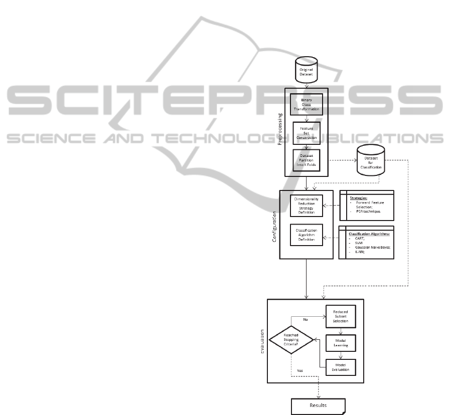
Figure 1 depicts the process performed for each
group of experiments.
Conceptually, our experimental process has three
major stages: preprocessing, configuration, and
evaluation. The first stage prepares the data for the
next stages; the second one defines the settings of
both dimensionality reduction strategy and
classification algorithm, and the last stage trains and
evaluates the learning model over the reduced
datasets.
All the stages were developed in Python and
were based on Scikit-learn (Pedregosa et al, 2011), a
well known machine learning library, and on
NetworkX (Hagberg et al., 2008) a development
environment frequently used to implement and
process graph structures.
2.3.1 Pre-processing
This stage is performed only once for each dataset. It
randomly selects samples from the original data in
order to build a dataset for the classification task.
The new dataset is the one used by the other stages.
This stage has the following steps:
a) Binary Class Transformation: this step is
responsible for taking a sample from the original
dataset modelled as a graph G and turning it into
a dataset formed by the pairs of vertices and their
classes. Each of the randomly selected pairs of
vertices is classified as positive or negative. The
classification process will depend on the kind of
task performed: for the future link prediction, the
original dataset is divided into two range of years
(Hasan et al., 2006) – the training years (which
represents the “present” period of time, and is
represented by the graph G
t
, originated from the
graph G), and the test years (which represents the
“future” period of time, and is represented by the
graph G
t+1
, also originated from the graph G). A
selected pair of vertices cannot have a link
between them in the training range, but may or
may not have a link in the test range, being
classified as positive or negative example,
respectively. This process was used with the
DBLP dataset. For the missing link prediction
task, the sample is selected from the graph G,
and the pairs of vertices are classified as positive
or negative if they have a link between them or
not. However, once the positive examples are
selected, their links are removed from the graph
G
t
, which is a copy from the original graph G (in
order to simulate their absence and consider
them the “missing” links). This criterion was
applied to Amazon and Flickr datasets.
b) Feature Set Construction: after building the
sample, the features of each selected pair of
vertices are calculated. As we have used only
topological features for this work, the features
are calculated based on the graph structure G
t
(which can represent different versions of the
original graph G, depending on the task
performed). We normalized the features values
using the standard score (Hasan et al., 2006).
After normalized, the calculated features are
attached to the tuple corresponding to its pair of
vertices in the dataset for classification.
Figure 1: The sequence of stages and their steps performed
for each experiment.
c) Dataset Partition into K-Folds: this step divides
the dataset for the classification task into K
different folds, adding the index of the fold of
each pair of nodes to its corresponding tuple. The
purpose of keeping the folds previously defined
ICEIS2015-17thInternationalConferenceonEnterpriseInformationSystems
298

was to consider the same dataset partition for the
k-fold cross-validation process to be executed
with every classification algorithm.
2.3.2 Configuration
The data analyst uses this stage to select both the
dimensionality reduction strategy and the
classification algorithm (and its parameters to be
employed in the evaluation stage). This stage has the
following steps:
a) Dimensionality Reduction Strategy Definition: in
this step, the dimensionality reduction strategy
that will be used for future evaluation is chosen.
There are two available strategies: FFS and PCA.
The former has no parameter. For the latter, the
maximum number of principal components that
will be generated from the dataset must be
defined by the user.
b) Classification Algorithm Definition: this step is
responsible for defining the classification
algorithm and its configuration to be used in the
supervised learning process. The tested
algorithms and their configurations are listed in
section 2.4.
2.3.3 Evaluation
The supervised learning process and dimensionality
reduction strategy evaluation effectively happen in
this stage. As depicted in the figure 1, the evaluation
stage is iterative, executing its steps in a loop. If the
PCA technique is chosen as dimensionality
reduction strategy, this loop will perform until the
maximum number of principal components are
evaluated. Otherwise, the FFS will be used, and as it
is an incremental strategy, its loop will perform until
there is no improvement of precision of the built
predictive models. The results of this stage are the
precision of the most accurate predictive model and
the number of principal components or features
(depending on the strategy) used to build this model.
This stage has the following steps:
a) Reduced Dataset Selection: this step applies the
dimensionality reduction strategy in the pre-
processed dataset, creating the reduced datasets.
If the FFS strategy is selected, at its first
iteration, a reduced dataset with each attribute of
the original feature set will be generated.
However, if the PCA technique is selected, there
will be as many reduced datasets as the
previously defined maximum number of
principal components.
b) Model Learning: In order to obtain a predictive
model, this step applies the classification
algorithm to the reduced dataset produced by the
previous step. The predefined configuration of
the algorithm is always used during the process.
As we are using the k-fold cross validation, we
build k different predictive models for each
reduced dataset. We have parallelized this
process, building these predictive models
simultaneously.
c) Model Evaluation: the predictive model is
evaluated in this step. All the k predictive models
are evaluated using the traditional k-fold cross
validation. We have used the precision of the
classification model to evaluate the reduced
dataset. As mentioned before, the validation was
parallelized, so the evaluation of each predictive
model happens simultaneously, and the final
precision is the average precision of these
predictive models.
2.4 Classification Algorithms
Although there are many classification algorithms
for supervised learning, we had to choose some of
them to perform our experiments. Summarized in
Table 1, our choices followed the ones reported in
(Hasan et al., 2006).
We performed some preliminary experiments
with each dataset, in order to set the parameter
values depicted in Table 2. For example, we ranged
k of k-NN from 3 to 9 in order to choose the one
(k=5) with the best classification results in the
evaluated datasets. Once set, such configurations
were used in all experiments.
Table 2: Classification algorithms used in this work.
Algorithm Comment
SVM
‘RBF’ Kernel; penalty = 100; kernel coeff.
= 0.1
K-NN K=5
Naïve Bayes (NB) Gaussian Distribution
CART Random State = 10
3 RESULTS AND DISCUSSIONS
We performed three groups of experiments. Each
group considered one of the three datasets. For the
future link prediction task in the DBLP dataset, we
have used a period of time from 1990 to 2000 as the
training years, and from 2001 to 2005 as test years.
As we have used the Amazon and Flickr datasets for
the missing link prediction task, we did not have to
define a period of time for them. We preprocessed
DimensionalityReductionforSupervisedLearninginLinkPredictionProblems
299

each dataset only once, at the beginning of the
experiments of its group. Then, we have applied
PCA, FFS and CS strategies with each classification
algorithm in each dataset using the 10-fold cross
validation process. The CS (Complete Set)
“strategy” was considered our baseline. It always
used the complete set of attributes (15 features). In
fact, no dimensionality reduction was performed
with it. With PCA, we have used 14 as the
maximum number of principal components for each
dataset. The FFS strategy demanded no parameter.
We have built a total of 5280 predictive models.
Table 3 summarizes our results. Each triple (dataset,
dimensionality reduction strategy, classification
algorithm) defines a cell that contains two numbers.
The first one is the average precision (%) of the
classification models produced by the subset of
experiments that applied the corresponding
dimensionality reduction strategy to the respective
classification algorithm and dataset during the 10-
fold cross validation process. The second one
(presented between brackets) indicates the number
of features (or principal components) of the most
precise classification model produced in such subset
of experiments.
The FFS strategy outperformed CS in eight of
twelve cases (66.6%). Only in the subset of
experiments with the Amazon dataset and SVM
algorithm, FFS presented the same average precision
of CS, but with a smaller feature subset. The PCA
outperformed CS in half of the cases (50%), having
the same average precision in three of them.
FFS overcame PCA in nine of twelve cases
(75%), while PCA only overcame FS in two of all
cases (16.6%).
It is worth to mention the improvement of the
Gaussian Naïve Bayes (NB) algorithm when
evaluated with a reduced dimension space. Not
surprisingly, for all datasets, this algorithm
performed much better with less correlated attributes
or principal components than with the complete
original feature set.
4 CONCLUSIONS
Link prediction is an important task in the scenario
of complex networks and supervised learning is an
approach to deal with it. High dimensionality is one
major problem in machine learning applications.
And so it is in the supervised learning link prediction
task. In spite of the importance of this problem, just
a few works related to dimensionality reduction in
link prediction have been developed. However, none
of them have used classical techniques from the
machine learning literature, such as principal
components analysis (PCA) and forward feature
selection (FFS).
Table 3: Summary of results obtained with the three
groups of experiments.
Dataset
Algorithm
Dimensionality Reduction Strategy
CS (%) FFS (%) PCA (%)
DBLP
CART 73.7 [15] 79.9 [02] 73.6 [10]
SVM 81.3 [15] 81.2 [07] 81.3 [11]
K-NN 80.0 [15] 79.2 [04] 80.1 [10]
NB 64.2 [15] 80.5 [05] 78.0 [01]
Amazon
CART 96.4 [15] 97.3 [03] 95.8 [04]
SVM 97.5 [15] 97.5 [07] 97.5 [11]
K-NN 97.2 [15] 97.5 [04] 97.3 [09]
NB 91.8 [15] 97.0 [03] 92.9 [03]
Flickr
CART 89.5 [15] 89.2 [02] 77.3 [07]
SVM 82.6 [15] 83.7 [03] 82.6 [10]
K-NN 79.2 [15] 86.4 [06] 79.8 [08]
NB 65.5 [15] 79.3 [01] 71.0 [04]
In this paper, we have explored the effects of
dimensionality reduction in the link prediction task,
by applying the traditional techniques of PCA and
FFS. The main contributions of our experiments
include: (a) results that showed that traditional
dimensionality reduction techniques can lead to
more precise and compact models in link prediction;
(b) the use of open datasets (which makes it easier
for other researchers to reproduce the experiments)
that cover “future” (DBLP) as well as “missing”
(Amazon and Flickr) link prediction applications; (c)
insertion of some topological measures (the last
three ones described in subsection 2.2) not usually
employed in link prediction state of art to describe
the datasets.
As future work, we consider the use and
evaluation of other classical feature selection
techniques in link prediction, including optimization
meta-heuristics, such as genetic algorithms. It would
be also interesting to use other datasets that include
not only the topological information, but information
from the graph nodes as well, in order to consider a
wider range of features. Experiments with other
classification algorithms for those link prediction
tasks and the use of other evaluation measures such
as recall, F-measure and AUC are also desirable.
ICEIS2015-17thInternationalConferenceonEnterpriseInformationSystems
300

ACKNOWLEDGEMENTS
This work has been partially supported by CNPq
(307647/2012-9), FAPERJ (E- 26/111.147/2011)
and CAPES (MSc scholarship).
REFERENCES
Adamic, L. A., Adar, E., 2003. Friends and neighbors on
the web. Social Networks, 25 (3), 211-230.
Barabasi, A. L., Jeong, H., Neda, Z., Ravasz, E., 2002.
Evolution of the social network of scientific
collaboration. Physica A: Statistical Mechanics and its
Applications, 311 (3), 590-614.
Barrat, A., Barthelemy, M., Pastor-Satorras, R. and
Vespignani, A., 2004. The architecture of complex
weighted networks. Proceedings of the National
Academy of Sciences, 101. 3747-3752.
Benchettara, N., Kanawati, R., Rouveirol, C., 2010.
Supervised Machine Learning applied to Link
Prediction in Bipartite Social Networks. International
Conference on Advances in Social Networks Analysis
and Mining, 326-330.
Caruana, R., Karampatziakis, N., Yessenalina, A., 2008.
An empirical evaluation of supervised learning in high
dimensions. International Conference on Machine
Learning (ICML). ACM. 96-103.
Freeman, L. C., 1978. Centrality in social networks
conceptual clarification. Social Networks, 1 (3).
Freitas, A. A., 2002. Data Mining and Knowledge
Discovery with Evolutionary Algorithms, Springer.
New York.
Hagberg, A. A., Schult, D. A., Swart, P. J., 2008.
Exploring network structure, dynamics, and function
using NetworkX. Proceedings of the 7th Python in
Science Conference (SciPy2008). 11-15.
Hasan, M. A., Chaoji, V., Salem, S., Zaki, M., 2006. Link
Prediction using Supervised Learning In Proc. of SDM
06 workshop on Link Analysis, Counterterrorism and
Security, Counterterrorism and Security, SIAM Data
Mining Conference.
Hasan, M. A., Zaki, M. J., 2011. A survey on Link
Prediction in Social Networks. Social Network Data
Analytics. Springer. 243-275.
Huang, Z., Li, X., Chen, H., 2005. Link prediction
approach to collaborative filtering. Proceedings of the
5th ACM/IEEE-CS joint conference on Digital
libraries. ACM. 141-142.
Izudheen, S., Mathew, S., 2013. Link Prediction in
Protein Networks. Indian Journal of Applied
Research, 3 (5).
Jackson, J. E., 1991. A User's Guide to Principal
Components, Wiley. New York.
Katz, L., 1953. A new status index derived from
sociometric analysis. Psychometrika, 18 (1). 39-43.
Kohavi, R., John, G. H., 1997. Wrappers for feature subset
selection. Artificial Intelligence, 97 (1). 273-324.
Leicht, E. A., Holme, P., Newman, M. E. J., 2006, Vertex
similarity in networks. Physical Review E, 73 (2).
Li, X., Chen, H., 2009. Recommendation as link
prediction: a graph kernel-based machine learning
approach. Proceedings of the 9th ACM/IEEE-CS joint
conference on Digital libraries. 213-216.
Liben-Nowell, D., Kleinberg, J., 2003. The link prediction
problem for social networks. Proceedings of the
twelfth international conference on Information and
knowledge management. 556-559.
Lind, P. G., Gonzalez, M. C., Herrmann, H. J., 2005.
Cycles and clustering in bipartite networks. Physical
Review E, 72.
Leskovec, J., Krevl, A., 2014. SNAP Datasets: Stanford
Large Network Dataset Collection. Retrieved from:
http://snap.stanford.edu/data.
Ley, M., 2009. DBLP: some lessons learned. Proceedings
of the VLDB Endowment, 2 (2).
Lü, L., Jin, C., Zhou, T., 2009. Similarity index based on
local paths for link prediction of complex networks. In
Physical Review, 80.
Lü, L., Zhou, T., 2011. Link prediction in complex
networks: A survey. Physica A, 390.
Narang, K.; Lerman, K. & Kumaraguru, P., 2013.
Network flows and the link prediction problem.
Proceedings of the 7th Workshop on Social Network
Mining and Analysis.
Oyama, S., Hayashi, K., Kashima, H., 2011, Cross-
temporal Link Prediction. Proceedings of the 11th
International Conference on Data Mining (ICDM).
Papadimitriou, A., Symeonidis, P., Manolopoulos, Y.,
2012. Fast and Accurate Link Prediction in Social
Networking Systems. Journal of Systems and
Software, 85 (9).
Pedregosa, F., Varoquaux, G., Gramfort, A., Michel, V.,
Thirion, B., Grisel, O., Blondel, M., Prettenhofer, P.,
Weiss, R., Dubourg, V., VanderPlas, J., Passos, A.,
Cournapeau, D., Brucher, M., Perrot, M., Duchesnay,
E., 2011. Scikit-learn: Machine Learning in Python.
Journal of Machine Learning Research, 12.
Pujari, M., Kanawati, R., 2012. Tag Recommendation by
Link Prediction Based on Supervised Machine
Learning. Proceedings of the Sixth International
Conference on Weblogs and Social Media.
Sa, H. R., Prudencio, R. B. C., 2011. Supervised link
prediction in weighted networks. The 2011
International Joint conference on Neural Networks
(IJCNN).
Saramäki, J.; Kivelä, M.; Onnela, J.; Kaski, K. & Kertesz,
J., 2007. Generalizations of the clustering coefficient
to weighted complex networks. Physical Review, 75
(2).
Shojaie A., 2013. Link Prediction in Biological Networks
using Penalized Multi-Mode Exponential Random
Graph Models. Proceedings of the 13th KDD
Workshop on Learning and Mining with Graphs.
Symeonidis, P., Iakovidou, N., Mantas, N.,
Manolopoulos, Y., 2013. From biological to social
networks: Link prediction based on multi-way spectral
clustering. Data & Knowledge Engineering, 87.
DimensionalityReductionforSupervisedLearninginLinkPredictionProblems
301

Wang, L., Hu, K., Tang, Y., 2013. Robustness of Link-
prediction Algorithm Based on Similarity and
Application to Biological Networks. Current
Bioinformatics, 9 (3).
Xu, Y., Rockmore, D., 2012. Feature selection for link
prediction. Proceedings of the 5th Ph.D. workshop on
Information and knowledge. 25-32.
Yu, L., Liu, H., 2003. Feature selection for high-
dimensional data: a fast correlation-based filter
solution. Machine Learning International Workshop
Then Conference, 20 (2).
ICEIS2015-17thInternationalConferenceonEnterpriseInformationSystems
302
