Plane-Sweep Algorithms for the K Group Nearest-Neighbor Query

George Roumelis

, Michael Vassilakopoulos

, Antonio Corral

and Yannis Manolopoulos

Department of Informatics, Aristotle University, GR-54124 Thessaloniki, Greece

Department of Electrical and Computer Engineering, University of Thessaly, GR-38221 Volos, Greece

Department of Informatics, University of Almeria, 04120 Almeria, Spain

groumeli@csd.auth.gr, mvasilako@uth.gr, acorral@ual.es, manolopo@csd.auth.gr

Keywords:

Spatial Query Processing, Plane-Sweep, Group Nearest-Neighbor Query, Algorithms.

Abstract:

One of the most representative and studied queries in Spatial Databases is the (K) Nearest-Neighbor (NNQ),

that discovers the (K) nearest neighbor(s) to a query point. An extension that is important for practical ap-

plications is the (K) Group Nearest Neighbor Query (GNNQ), that discovers the (K) nearest neighbor(s) to a

group of query points (considering the sum of distances to all the members of the query group). This query

has been studied during the recent years, considering data sets indexed by efﬁcient spatial data structures. We

study (K) GNNQs, considering non-indexed data sets, since this case is frequent in practical applications. And

we present two (RAM-based) Plane-Sweep algorithms, that apply optimizations emerging from the geometric

properties of the problem. By extensive experimentation, using real and synthetic data sets, we highlight the

most efﬁcient algorithm.

1 INTRODUCTION

Spatial database is a database that offers spatial data

types (for example, types for points, line segments,

regions, etc.), a query language with spatial predi-

cates, spatial indexing techniques and efﬁcient pro-

cessing of spatial queries (Rigaux et al., 2002). It has

grown in importance in several ﬁelds of application

such as urban planning, resource management, trans-

portation planning, etc. Together with them come

various types of complex queries that need to be an-

swered efﬁciently.

One of the most representative and studied queries

in Spatial Databases is the (K) Nearest-Neighbor

Query (NNQ), that discovers the (K) nearest neigh-

bor(s) to a query point. An extension that is impor-

tant for practical applications is the (K) Group Near-

est Neighbor Query (GNNQ), that discovers the (K)

nearest neighbor(s) to a group of query points (con-

sidering the sum of distances to all the members of

the query group). This query has been studied during

the recent years, considering data sets indexed by efﬁ-

cient spatial data structures. An example of its utility

could be when we have a set of meeting points (data

set) and a set of user locations (query set), and we

want to ﬁnd the set of one (K) meeting point(s) that

minimizes the sum of distances for all user locations,

since each user will travel from his location to each

of the K meeting points. More speciﬁcally, user lo-

cations may represent residence locations and meet-

ing points may represent points of interest (cultural

landmarks). Each of the K points is visited by each

user for whole day inspection and the user returns to

his residence overnight, before visiting the next land-

mark on the following day. We may interested to

solve such a problem for a speciﬁc pair of data and

query sets only once, but we may face several such

problems for different pairs of sets. Note that, buid-

ing indexes for the data sets would be needed only if

several queries would be answered for the these data

sets, which might evolve gradually in the course of

time and not be completely replaced by new data sets.

One of the most important techniques in the com-

putational geometry ﬁeld is the Plane-Sweep (PS) al-

gorithm, which is a type of algorithm that uses a con-

ceptual sweep line to solve various problems in the

Euclidean plane, E

, (Preparata and Shamos, 1985).

The name of PS is derived from the idea of sweep-

ing the plane from left to right with a vertical line

(front) stopping at every transaction point of a geo-

metric conﬁguration to update the front. All process-

ing is done with respect to this moving front, without

any backtracking, with a look-ahead on only one point

each time (Hinrichs et al., 1988). For instance, the

PS technique has been successfully applied in spatial

query processing, mainly for intersection joins (Jacox

Roumelis G., Vassilakopoulos M., Corral A. and Manolopoulos Y..

Plane-Sweep Algorithms for the K Group Nearest-Neighbor Query.

DOI: 10.5220/0005375300830093

In Proceedings of the 1st International Conference on Geographical Information Systems Theory, Applications and Management (GISTAM-2015), pages

83-93

ISBN: 978-989-758-099-4

 2015 SCITEPRESS (Science and Technology Publications, Lda.)

and Samet, 2007).

In (Roumelis et al., 2014), the problem of process-

ing K Closest Pair Query between RAM-based point

sets was studied, using PS algorithms. Two improve-

ments that can be applied to a PS algorithm and a

new algorithm that minimizes the number of distance

computations, in comparison to the classic PS algo-

rithm, were proposed. By extensive experimentation,

using real and synthetic data sets, the most efﬁcient

improvement was highlighted and it was shown that

the new PS algorithm outperforms the classic one.

In this paper, we study (K) GNNQs, considering

non-indexed data sets (a frequent case in practical ap-

plications, see the example given previously), unlike

previous research presented in Section 2 that consider

that both data sets are indexed by structures of the

R-tree family. Our target is to design efﬁcient non-

index based algorithms for (K) GNNQs and highlight

the most efﬁcient among them. Thus, we present two

(RAM-based) PS algorithms, that apply optimizations

emerging from the geometric properties of the prob-

lem. Several experiments have been performed, using

real and synthetic data sets, to show the most efﬁcient

algorithm. In the future, we plan to compare the best

of our algorithms to existing index based solutions.

The paper is organized as follows. In Section 2,

we review the related literature and motivate the re-

search reported here. In Section 3, two new PS al-

gorithms for GNNQs are presented. In Section 4, a

comparative performance study is reported. Finally,

in Section 5, conclusions on the contribution of this

paper and future work are summarized.

2 RELATED WORK AND

MOTIVATIONS

GNN queries are introduced in (Papadias et al., 2004)

and it consist in given two sets of points P and Q,

a GNN query retrieves the point(s) of P with the

smallest sum of distances to all points in Q. GNN

queries are also known as aggregate nearest neighbor

(ANN) queries (Papadias et al., 2005). In (Papadias

et al., 2004), the authors have developed three differ-

ent methods were developed, MQM (multiple query

method), SPM (single point method) and MBM (min-

imum bounding method), to evaluate a GNN query

that minimizes the total distance from a set of query

points to a data point. In (Papadias et al., 2005) these

methods have been extended to minimize the mini-

mum and maximum distance in addition to the total

distance with respect to a set of query points. All

these methods assume that the data points are indexed

using an R-tree and can be implemented using both

depth-ﬁrst search and best-ﬁrst search algorithms.

In general terms, MQM performs an incremental

search for the nearest data point of each query point

in the set and compute the aggregate distance from

all query points for each retrieved data point. The

search ends when it is ensured that the aggregate dis-

tance of any non-retrieved data point in the database is

greater than the current K-th minimum aggregate dis-

tance, that is the K GNNs are found. It means MQM

is a threshold algorithm, since it computes the nearest

neighbor for each query point incrementally, updat-

ing different thresholds according to the target of the

KGNN. The main disadvantage of MQM is that it tra-

verses the R-tree multiple times and it can access the

same data point more than once.

The other methods, SPM and MBM, ﬁnd the K

GNNs in a single traversal of the R-tree. SPM ap-

proximates the centroid of the query distribution area

and continues the searching with respect to the cen-

troid until the current KGNNs are determined. Dur-

ing the search, some heuristics based on triangular

inequality are used to prune intermediate nodes and

determine the real nearest neighbors to Q. MBM re-

gards Q as a whole and uses its MBR M to prune the

search space in a single query, in either a depth-ﬁrst

or best-ﬁrst manner. Moreover, two pruning heuristics

involving the distance from an intermediate node to M

or query points are proposed and they can be used in

either traversal policy. Experimental results showed

that the performance of MBM is better than SPM and

MQM for memory and disk resident queries, since

it traverses the R-tree once and takes the query dis-

tribution area into account. Moreover, according to

the comparison conducted in (Papadias et al., 2004),

MBM is better than SPM in terms of node access and

CPU cost while MQM is the worst.

In (Li et al., 2005), the authors propose two prun-

ing strategies for KGNN queries which take into ac-

count the distribution of query points. Such methods

employ an ellipse to approximate the extent of mul-

tiple query points, and then derive a distance or min-

imum bounding rectangle using that ellipse to prune

intermediate nodes in a depth-ﬁrst search via an R

∗

tree. These methods are also applicable to the best-

ﬁrst traversal. The experimental results show that the

proposed pruning strategies are more efﬁcient than the

methods presented in (Papadias et al., 2004).

A new method to evaluate a KGNN query for non-

indexed data points using projection-based pruning

strategies was presented in (Luo et al., 2007). Two

points projecting-based ANNQ algorithms were pro-

posed, which can efﬁciently prune the data points

without indexing. This new method projects the query

points into a special line, on which their distribution

GISTAM2015-1stInternationalConferenceonGeographicalInformationSystemsTheory,ApplicationsandManagement

is analysed, for pruning the search space.

In (Namnandorj et al., 2008), a new property in

vector space was proposed and, based on it some efﬁ-

cient bound estimations were developed for two most

popular types of ANN queries (sum and maximum).

Taking into account these bounds, indexed and non-

index ANN algorithms were designed. The proposed

algorithms showed interesting results, especially for

high dimensional queries.

Other related contributions in this research line

have been proposed in the literature. In (Hashem

et al., 2010) an efﬁcient algorithm for KGNN query

considering privacy preserving was proposed, and the

existing KGNN algorithms (Papadias et al., 2005)

for point locations were extended to regions in or-

der to preserve user privacy. In (Zhu et al., 2010),

the KGNN query in road networks based on network

voronoi diagram was solved. In (Jiang et al., 2013),

the reverse top-K group nearest neighbor search is

presented. In (Zhang et al., 2013), the KNN and

KGNN queries are extended to get a new type of

query, so-called K Nearest Group (KNG) query. It

retrieves closest elements from multiple data sources,

and it ﬁnds K groups of elements that are closest to

a given query point, with each group containing one

object from each data source. And recently, for uncer-

tain databases, probabilistic KGNN query was studied

by (Lian and Chen, 2008; Li et al., 2014).

Therefore, the KGNN is an active research line

nowadays and most of the contributions have used in-

dexes (of the R-tree family) for their solutions. The

main motivation of this paper is to use the Plane-

Sweep technique to solve the problem proposed in

(Papadias et al., 2004), when neither of the inputs

are indexed. Due to not using indexes, the algorithms

proposed in this paper are completely different to pre-

vious solutions. To the best of our knowledge, there

are not any existing solutions for the (K) GNNQ with-

out indexes. The unnecessity of indexes is not in-

frequent in practical applications, when the data sets

change at a very rapid rate, or the data sets are not

reusable for subsequent queries (see the example in

Section 1).

3 PLANE-SWEEP ALGORITHMS

FOR GNNQ

In this section we introduce two Plane-Sweep algo-

rithms for processing GNNQ. The input of this query

consists of a set P = {p

, p

,··· , p

N−1

} of static data

points in the Euclidean plane, E

, and a group of

query points Q = {q

,··· , q

M−1

}. The output

contains the K (≥ 1) data point(s) with the small-

est sum of distances to all points in Q. The dis-

tance between a data point p ∈ P and Q is deﬁned as

sumdist(p, Q) =

∑

M−1

i=0

dist(p, q

), where dist(p, q

) is

the Euclidean distance between p ∈ P and a query

point q

∈ Q. A simple application of Plane-Sweep,

assuming that both data sets are sorted in ascending

order of their X -values, would compute the sum of

distances of each data point to all the query points, by

examining the data points from left to right, along the

sweeping axis (e.g. X-axis). In the following we will

denote the sum of distances (dx-distances) of a data

point p to the set of query points Q by sumdist(p, Q)

(sumdx(p, Q)). Note that, while the sweep line ap-

proaches (moves away from) the median point(s),

sumdx will be decreasing (increasing). This is proved

in the Appendix. And, sumdx(p, Q) ≤ sumdist(p, Q),

for a data point p ∈ P. Besides, we must empha-

size that dx-distance (dx dist(p,q), ∆x(p,q)) is the

distance function between two points p and q over

the X -axis, an analogous expression is for dy-distance

(dy dist(p, q), ∆y(p,q)) over the Y-axis. And the

sum of dx-distances between one given point p ∈ P

and all query points of Q (q

∈ Q) is deﬁned as

sumdx(p, Q) =

∑

M−1

i=0

dist(p, q

A max binary heap (keyed by sumdist and called

MaxKHeap) that keeps the K data points with the

smallest sum of distances to the query points found so

far is used. The sumdist of the root of the MaxKHeap

is denoted by δ. In case the heap is not full (it contains

less than K points), p will be inserted in the heap, re-

gardless of sumdist(p,Q). Otherwise, for each data

point p being compared with the query set Q, there

are 2 cases:

1. Case 1: If sumdx(p,Q) is larger than or equal to

δ, then there is no need to calculate sumdist(p, Q)

(rule 1).

2. Case 2: If the sumdist(p,Q) is smaller than δ,

then p will be inserted in the heap (rule 2).

Let p with sumdx(p, Q) ≥ δ, then, for every

with p

.x ≥ p.x, sumdx(p

,Q) ≥ sumdx(p, Q).

Moreover, sumdist(p

,Q) ≥ sumdx(p

,Q). Thus,

sumdist(p

,Q) ≥ δ and we do not need to calculate

any distance for p

In the algorithms that we have developed, we ﬁnd

a data point p

∈ P that is X-closest to the median

point of the query set Q (in case that the query set

contains an even number of points, we choose the

right of the two median points). This data point is

found by binary search. The sweep line is located

on p

i−1

and moves to left until a data point p with

sumdx(p, Q) ≥ δ is found (termination condition 1).

Then, the sweep line is located on p

and moves to

the right until a data point p with sumdx(p, Q) ≥ δ

(termination condition 2). At this stage, MaxKHeap

Plane-SweepAlgorithmsfortheKGroupNearest-NeighborQuery

Algorithm 1: GNNPS.

Input: Two X-sorted arrays of points P = {p[0], p[1],· ·· , p[N − 1]}, Q = {q[0], q[1],··· ,q[M − 1]}, and MaxKHeap.

Output: MaxKHeap storing the K Nearest Neighbors having smallest sums of distances to all query points.

1: i = f ind closest point(P, q[m])  STEP 1 : Preperation. q[m] is the median point of query set Q.

2: j = i − 1

3: while j > −1 do  STEP 2 : Search in the range p[ j].x ≤ q[m].x, descending j

4: if calc sum dist(p[ j − −], Q,MaxKHeap) == err code dx then  Termination condition 1

5: break

6: while i < N do  STEP 3 : Search in the range p[i].x > q[m].x, ascending i

7: if calc sum dist(p[i + +],Q,MaxKHeap) == err code dx then  Termination condition 2

8: break

Algorithm 2: calc sum dist.

Input: One point p, the sorted array of query points Q = {q[0],q[1], ··· ,q[M − 1]}, and MaxKHeap.

Output: Value success f ul insertion or err code dx or err code dist and MaxKHeap updated with p if rule 2 was true.

1: function calc sum dist(p, Q, MaxKHeap)

2: sumdist = 0.0, sumdx = 0.0

3: if MaxKHeap is not f ull then

4: for k = 0;k < M; k + + do  for each query point q

5: sumdist+ = dist(p,q[k])  dist() computes the Euclidean distance between p and q[k]

6: MaxKHeap.insert(p,sumdist)

7: return sucess f ul insertion

8: else

9: for k = 0;k < M; k + + do  for each query point q

10: sumdx+ = dx dist(p,q[k])  dx dist() computes the dx-distance between p and q[k] (∆x(p, q[k]))

11: if sumdx ≥ MaxKHeap.root.dist then  Rule 1

12: return err code dx  exit k, all other points have longer distance

13: for k = 0;k < M; k + + do  for each query point q

14: sumdist+ = dist(p,q[k])  add the distance (dist) from the current point

15: if sumdist < MaxKHeap.root.dist then  Rule 2

16: MaxKHeap.insertFull(p,sumdist)

17: return sucess f ul insertion

18: else

19: return err code dist  not inserted because of sum of distances (sumdist)

will contain the K data points with the smallest sum

of distances to the query points.

In (Papadias et al., 2004) it was proved that

for every data point p with |Q| · dist(p,c) ≥ δ +

sumdist(c, Q), p can be ignored, without calculating

any distance. In the second algorithm that we have de-

veloped, the centroid c of the query points is also used

and the above condition is a pruning condition for

points that saves a signiﬁcant number of calculations.

Moreover, in the second algorithm, when the sweep

line is outside of the area of query points, then for the

current data point p, sumdx(p, Q) = |Q| · |p.x − c.x|.

Using this condition, we save numerous calculations.

In the Appendix, we prove that the sum of dx-

distances between one given point p(x, y) ∈ P and all

points of the query set Q (sumdx(p, Q)):

A Is minimized at the median point q[m] (where q[m]

is the array notation of q

B For all p.x ≥ q[m].x, sumdx is constant or increas-

ing with the increment of x, and

C For all p.x < q[m].x, sumdx is increasing while x

decreases.

The ﬁrst algorithm (that is only based on median)

is called GNNPS and it uses the helper algorithm

calc sum dist and the function f ind closest point.

Firstly, it calculates the initial position of the sweep-

ing line (preparation state). For this, the algorithm

must ﬁnd the ﬁrst point p[i] ∈ P which is on the right

of the median of query set q[m] (p[i].x > q[m].x), by

calling the function f ind closest point (line 1). After

this, the algorithm sets the sweeping line at the point

p[i − 1] (line 3) and continues scanning the points of

set P decreasing the index i until the termination con-

dition 1 will be true or the points of set p will have ﬁn-

ished (lines 3-5). Lastly, the algorithm sets the sweep-

ing line at the point p[i] and continues scanning the

points of set P increasing the index i until the termi-

nation condition 2 will be true or the points of the set

P will have ﬁnished (lines 6-8).

The second algorithm (that is based on median and

centroid) is called GNNPSC and it uses the helper

GISTAM2015-1stInternationalConferenceonGeographicalInformationSystemsTheory,ApplicationsandManagement

Algorithm 3: GNNPSC.

Input: Two X-sorted arrays of points P = {p[0], p[1],· ·· , p[N − 1]}, Q = {q[0], q[1],··· ,q[M − 1]}, and MaxKHeap.

Output: MaxKHeap storing the K Nearest Neighbors having smallest sums of distances to all query points.

1: i = f ind closest point(P, q[m])  STEP 1 : Preperation. q[m] is the median point of query set Q.

2: j = i − 1

3: c(x,y) = Calculate Centroid coord(Q)  calculate the coordinates of the Centroid

4: sumdistCQ = 0.0

5: for k = 0; k < M;k + + do  for each query point q

6: sumdistCQ+ = dist(c, q[k])

 STEP 2 : Search in the range p[ j].x ≤ q[m].x, descending j

7: cont search = true  initialize the ﬂag

8: while j > −1 and p[ j].x > q[0].x do  for each point p[ j] inside the query MBR in sweeping axis (X-axis)

9: if calc sum dist in(p[ j − −], Q,c,sumdistCQ,MaxKHeap) == err code dx then  Termination condition 1

10: cont search = f alse

11: break

12: if cont search = true then

13: while j > −1 do  for each point p[ j] on the left of the query MBR in sweeping axis

14: if calc sum dist out(p[ j − −],Q, c,sumdistCQ, MaxKHeap) == err code dx then  Termination condition 1

15: break

 STEP 3 : Search in the range p[i].x > q[m].x, ascending i

16: cont search = true

17: while i < N and p[i].x < q[M − 1].x do  for each point p[i] inside the query MBR in sweeping axis

18: if calc sum dist in(p[i + +],Q,c,sumdistCQ,MaxKHeap) == err code dx then  Termination condition 2

19: cont search = f alse

20: break

21: if cont search = true then

22: while i < N do  for each point p[i] on the left of the query MBR in sweeping axis

23: if calc sum dist out(p[i + +],Q,c,sumdistCQ,MaxKHeap) == err code dx then  Termination condition 2

24: break

algorithms calc sum dist in and calc sum dist out

and the function f ind closest point. Firstly, the

algorithm calculates the initial position of the

sweeping line and the coordinates of the cen-

troid (preparation state). For these, the algorithm

calls the functions f ind closest point (line 1) and

Calculate Centroid coord(Q) (line 3). In the next

step, it continues scanning the points of set P decreas-

ing the index j until the termination condition 1 will

be true or the x-coordinate of the current point of set

P is smaller than or equal to the X -coordinate of the

ﬁrst query point q[0] (p[ j].x ≤ q[0]). In this state,

GNNPSC calls the function calc sum dist in to cal-

culate the sum of distances. After exiting the previous

loop and if the termination condition 1 has not arisen

(line 12), the algorithm continues decreasing j until

the termination condition 1 will be true or the points

of set P will have ﬁnished (lines 13-15). Lastly, the

algorithm sets the sweeping line at the point p[i] and

continues scanning the points of set P increasing the

index i just like in the previous step (lines 17-20 in-

side query set Q and lines 21-24 outside query set Q).

We must highlight that the function calc sum dist in

is the same as calc sum dist, adding two new param-

eters (the centroid of Q (c) and its sum of distances to

all query points (sumdistCQ)) and the following state-

ments just after the line 9.

9 : dist pc = calc dist(p, c)

10 : if M ·dist pc ≥ maxKheap.root.dist + sumdistCQ then

11 : return err code dist centroid

And the remaining statements of calc sum dist in

from line 12 (12-22) are the same as calc sum dist.

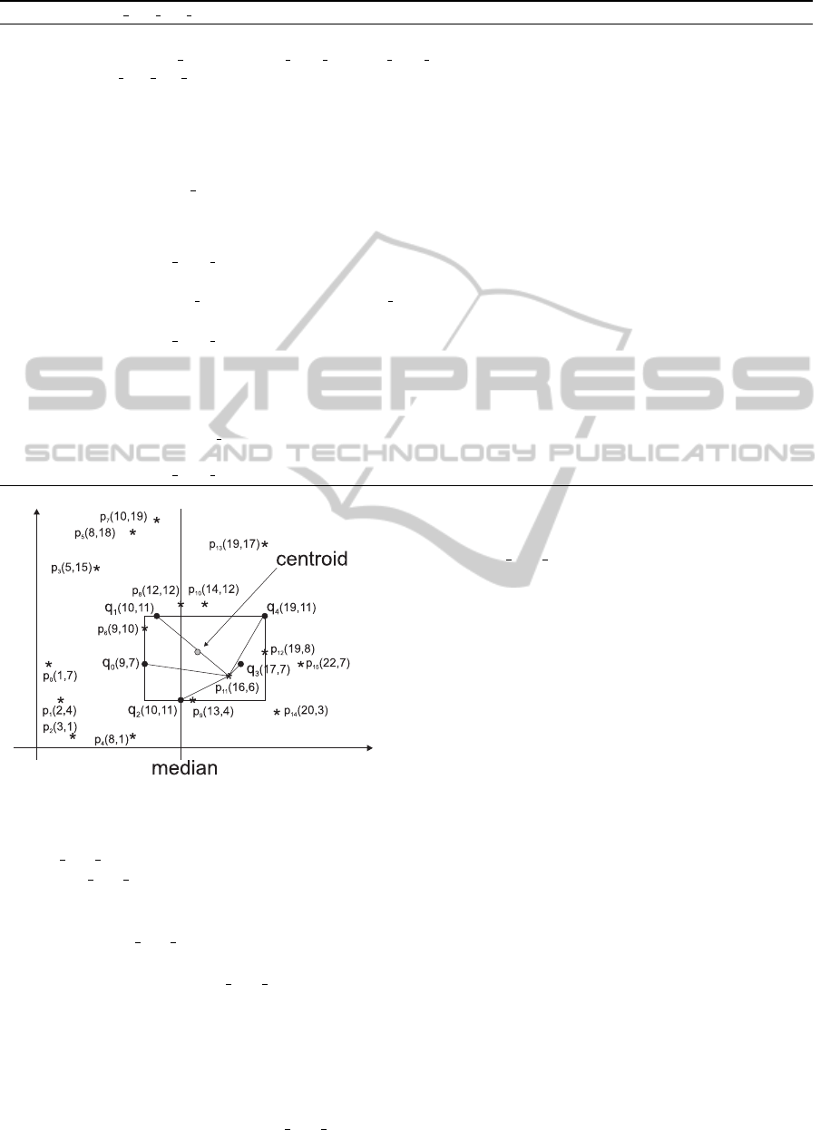
The following examples illustrate the execution

of the algorithms. The point data set P is deﬁned as

P = {p

(1,7); p

(2,4); p

(3,1); p

(3,13); p

(8,2);

(8,18); p

(9,10); p

(10,19); p

(12,12); p

(13,4);

(14,12); p

(16,6); p

(19,8); p

(19,17);

(20,3); p

(22,7) }, and the point query set Q

is deﬁned as Q = {q

(9,7); q

(10,11); q

(12,4);

(17,7); q

(19,11) }. In Figure 1, P and Q (they

are sorted in ascending order of their X -values), the

centroid and the median of the query points and the

initial position of the sweep line are drawn.

In GNNPS, ﬁrstly (in Step 1) the algorithm

searches for the point of the P set which is on

the right of the median q

(12,4) query point (line

1). That is p

(13,4) point. In Step 2 (lines 3-5)

it starts calculating the sum of distances between

point p

(12,12) and all query points. The result

is sumdist(p

,Q) = 30.209 and the point p

is in-

serted in the MaxKHeap (calc sum dist:lines 2-7).

In the next iteration the point p

(10,19) is examined.

The MaxKHeap is full and the second part of the

calc sum dist function (lines 9-19) is executed. The

sum of distances is sumdist(p

,Q) = 61.108 larger

than the MaxKHeap.root.dist = 30.209 (condition in

Plane-SweepAlgorithmsfortheKGroupNearest-NeighborQuery

Algorithm 4: calc sum dist in.

Input: One point p, set of query points Q, centroid c, its sum of distances to all query points sumdistCQ and MaxKHeap.

Output: Value success f ul insertion or err code dx or err code dist and MaxKHeap updated with p if rule 2 was true.

1: function calc sum dist in(p, Q, c, sumdistCQ, MaxKHeap)

2: sumdist = 0.0, sumdx = 0.0

3: if MaxKHeap is not f ull then

4: for k = 0;k < M; k + + do  for each query point q

5: sumdist+ = dist(p,q[k])  dist() computes the dx-distance between p and q[k]

6: MaxKHeap.insert(p,sumdist)

7: return sucess f ul insertion

8: else

9: d pc = dist(p,c)  dist() computes the distance between p and c

10: if M · d pc − sumdistCQ ≥ MaxKHeap.root.dist then  prune p without computing distances

11: return err

code dist;  not inserted because of sum of distances

12: for k = 0;k < M; k + + do  for each query point q

13: sumdx+ = dx dist(p,q[k])  dx dist() computes the dx-distance between p and q[k] (∆x(p, q[k]))

14: if sumdx ≥ MaxKHeap.root.dist then  Rule 1

15: return err code dx  exit k, all other points have longer distance

16: for k = 0;k < M; k + + do  for each query point q

17: sumdist+ = dist(p,q[k])  add the distance (dist) from the current point

18: if sumdist < MaxKHeap.root.dist then  Rule 2

19: MaxKHeap.insertFull(p,sumdist)

20: return sucess f ul insertion

21: else

22: return err code dist  not inserted because of sum of distances (sumdist)

Figure 1: The points of P and Q, the centroid, the median of

the query points and the initial position of the sweep line.

the calc sum dist:line 15 is false), so the point is re-

jected (calc sum dist:line 19). In the third iteration

the point p

(9,10) is examined and the sum of dis-

tances is sumdist(p

,Q) = 29.716 which is smaller

(condition of calc sum dist:line 15 is true) than the

MaxKHeap.root.dist therefore the point p

is in-

serted in the MaxKHeap (calc sum dist:lines 16,17)

by replacing the previous root (p

). In the fourth

and ﬁfth iterations for the points p

and p

the

sum of distances are sumdist(p

,Q) = 60.317 and

sumdist(p

,Q) = 43.299, respectively; both larger

than the MaxKHeap.root.dist and the points are

rejected. In the sixth iteration, the point p

has

sumdx(p

.x,Q) = 52 (condition in calc sum dist:line

11) which is larger than the MaxKHeap.root.dist

and the process (scanning the P set on the left)

ends (calc sum dist:line 12) because it is impossi-

ble to ﬁnd other points of set P on the left of p

having sum of distances smaller than 52. The al-

gorithm continues scanning the points of set P to

the right of the median q

, starting from the p

point. Its sumdist(p

,Q) = 27.835 is smaller than

the MaxKHeap.root.dist = 29.716 so it replaces

the existing point in the root of MaxKHeap. The

next point p

has sumdist(p

,Q) = 30.370 and it

is rejected. The next iteration will try the point

which has sumdist(p

,Q) = 26.599 the small-

est sum of distances and this point (p

) is in-

serted in the MaxKHeap replacing the previous root

. In the last iteration the algorithm examines

the point p

which has sumdx(p

,Q) = 28 larger

than the MaxKHeap.root.dist = 26.599 and the pro-

cess is ﬁnally ﬁnished. While executing this algo-

rithm we made 46 complete point-point distance cal-

culations, 84 point-point dx-distance calculations, 4

points with their sum of distances were inserted in the

MaxKHeap and 10 of the 16 points of set P were ex-

amined.

GNNPSC starts (Step 1) by ﬁnding the ﬁrst point

of set P which is on the right of the median point of

query set Q. That is the point p

. Afterwards it calcu-

lates the coordinates of centroid point c(x,y) = (13,8)

and then calculates the sum of distances between the

centroid and the query points sumdist(c,Q) = 23.374.

GISTAM2015-1stInternationalConferenceonGeographicalInformationSystemsTheory,ApplicationsandManagement

Algorithm 5: calc sum dist out.

Input: One point p, set of query points Q, centroid c, its sum of distances to all query points sumdistCQ and MaxKHeap.

Output: Value success f ul insertion or err code dx or err code dist and MaxKHeap updated with p if rule 2 was true.

1: function calc sum dist out(p, Q, c, sumdistCQ, MaxKHeap)

2: sumdist = 0.0, sumdx = 0.0

3: if MaxKHeap is not f ull then

4: for k = 0;k < M; k + + do  for each query point q

5: sumdist+ = dist(p,q[k])  dist() computes the dx-distance between p and q[k]

6: MaxKHeap.insert(p,sumdist)

7: return sucess f ul insertion

8: else

9: dx = dx dist(p,c)  dx dist() computes the dx-distance between p and c (∆x(p, c))

10: if M · dx ≥ MaxKHeap.root.dist then  Rule 1

11: return err code dx;  exit k, all other points have longer distance

12: dy = dy dist(p,c)  dy dist() computes the dy-distance between p and c (∆y(p,c))

13: dist pc =

+ dy

14: if M · dist pc ≥ MaxKHeap.root.dist + sumdistCQ then

15: return err code dist centroid;

16: for k = 0;k < M; k + + do  for each query point q

17: sumdist+ = dist(p,q[k])

18: if sumdist < MaxKHeap.root.dist then  Rule 2

19: MaxKHeap.insertFull(p,sumdist)

20: return sucess f ul insertion

21: else

22: return err code dist  not inserted because of sum of distances (sumdist)

GNNPSC continues with Step 2. In that step,

the points of set P are scanned on the left of the

in two particular steps. First from p

up to

which have X-coordinate larger than q

.x = 9

by calling the calc

sum dist in function. There

is sumdist(p

,Q) = 30.209 and this point is in-

serted in the MaxKHeap as the ﬁrst point while

the maxKHeap is empty (calc sum dist in:lines 3-

7). The point p

is examined next and it is rejected

without a need to calculate sumdist(p

,Q) because

the condition of the function calc sum dist in:line

10 is true. Step 2 continues scanning the points

of set P which are on the left (outside) of the q

query point by calling the function calc sum dist out.

The point p

with sumdist(p

,Q) = 29.716 is in-

serted (calc sum dist in:lines 9-20), while points p

and p

are rejected with sumdist(p

,Q) = 60.137

and sumdist(p

,Q) = 43.299 respectively, both larger

than the MaxKHeap.root.dist = 29.716 with the

point p

. The next point p

is the last point to be

examined because it has sumdx(p

,Q) = 52 larger

than the current MaxKHeap.root.dist. The algo-

rithm continues by executing Step 3, scanning the

points of set P on the right of the median query

point q

. The algorithm continues scanning the

points of set P to the right starting from the p

point. Its sumdist(p

,Q) = 27.835 is smaller than

the MaxKHeap.root.dist = 29.716 so it replaces the

existing point in the root of MaxKHeap. The next

point p

has sumdist(p

,Q) = 30.370 and it is re-

jected. The next iteration will try the point p

which

has sumdist(p

,Q) = 26.599 the smallest sum of dis-

tances and this point is inserted in the MaxKHeap re-

placing the previous root p

. In the last iteration we

examine the point p

which has sumdx(p

,Q) = 28

larger than the MaxKHeap.root.dist = 26.599 and

the process is ﬁnally ﬁnished. While executing this

algorithm we made 42 complete point-point distance

calculations, 38 point-point dx-distance calculations,

4 points with their sum of distances were inserted in

the MaxKHeap and 10 of 16 points of set P were ex-

amined.

4 EXPERIMENTATION

In order to evaluate the behaviour of the proposed

algorithms, we have used 6 real spatial data sets of

North America, representing cultural landmarks (CL

with 9203 points) and populated places (PP with

24493 points), roads (RD with 569120 line-segments)

and railroads (RR with 191637 line-segments). To

create sets of points, we have transformed the MBRs

of line-segments from RD and RR into points by tak-

ing the center of each MBR (i.e., |RD| = 569120

points, |RR| = 191637 points). Moreover, in order to

get the double amount of points from RR and RD, we

chose the two points with min and max coordinates of

the MBR of each line-segment (i.e. |RDD| = 1138240

points and |RRD| = 383274 points). The data of these

Plane-SweepAlgorithmsfortheKGroupNearest-NeighborQuery

6 ﬁles were normalized in the range [0, 1]

. The real

data sets we used are geographical. In order to test

the performance of our algorithms with data appear-

ing in Science, we have created synthetic clustered

data sets of 125000 (125K), 250000 (250K), 500000

(500K) and 1000000 (1000K) points, with 125 clus-

ters in each data set (uniformly distributed in the

range [0,1]

), where for a set having N points, N/125

points were gathered around the center of each cluster,

according to Gaussian distribution (this distibution is

common for natural properties of systems within Sci-

ence). The ﬁrst real data set (CL) was used to make

the query set (Q) by selecting the appropriate num-

ber of points randomly. Then the coordinates of these

points were appropriately scaled in order to get the

MBR of the query points to get a pre-deﬁned size in

comparison to the MBR of the data set (P). The other

9 data sets were used as data sets (P) within which we

were looking for the NNs.

All experiments were performed on a PC with In-

tel Core 2 Duo, 2.2 GHz CPU with 4 GB of RAM and

several GBs of secondary storage, with Ubuntu Linux

v. 14.04, using the GNU C/C++ compiler (gcc). The

performance measurements were: (1) the response

time (total query execution time) of processing the

(K) GNNQ, not counting reading from disk ﬁles to

main memory and sorting, (2) the number of points

involved in calculations, and (3) the number of X-axis

distance computations (dx-distance).

In every experiment the query set was moved on

X-axis in 8 equal size steps from the top left corner

of the area of the data set (P) up to the right corner

and after this, one step down on the Y -axis and so on.

The total execution time, and the other experimenta-

tion metrics, for each one experiment, were computed

as an average of all (the 64) queries.

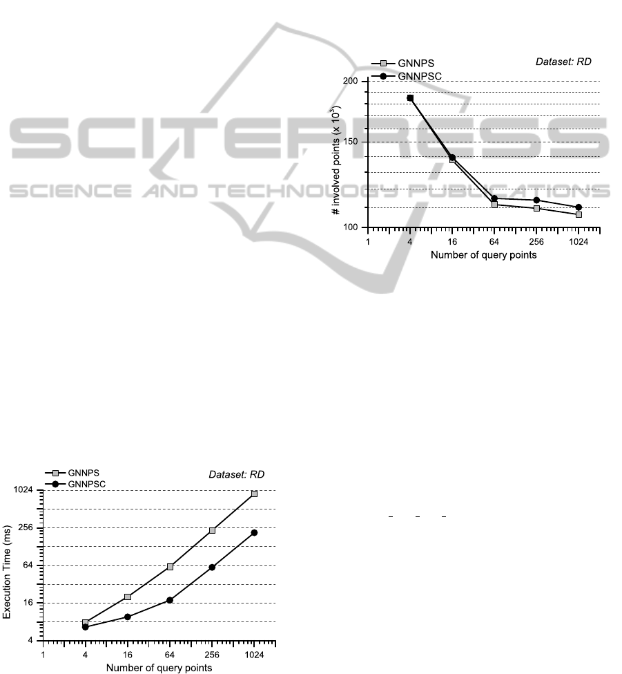
In Figure 2, we depict the effect of the number

of query points, N, on execution time of both al-

Figure 2: Execution time of the algorithms as a function of

N (RD data set).

gorithms for the RD data set (the number of group

nearest-neighbors, K, was equal to 8 and the size of

query-set MBR was 8% of the data set space). Anal-

ogous diagrams created for dx-distance and dist cal-

culations had similar appearance. It is obvious that

the increase of N leads to an increase of the execution

time, but with a smaller rate of increase. GNNPSC

needs less time than GNNPS, because of the use of

centroid (the computation of the distance between the

centroid and the reference point of set P needs one

calculation of distance while the computation of the

sum of distances between the reference point and all

query points needs N distance calculations).

Figure 3: # Points involved in calculations of the algorithms

as a function of N (RD data set).

For the same parameter settings and data set, in

Figure 3, we depict the effect of N on the number

of data set points involved in calculations. We ob-

serve that this number of points is reduced as N in-

creases. The sums of distances of the points of data

set P near the median are enlarged to a smaller ex-

tent, compared to the sumdist of the points outside

the MBR. This enables the termination conditions and

makes it possible to get nearest to the median query

point. Moreover, we can observe in Figure 3 that GN-

NPSC needs more involved points and from Figure 2

it is the fastest. This behaviour could be due to that in

function calc sum dist in we ﬁrstly apply the pruning

condition of centroid and next the termination condi-

tion 1 or 2 is checked. So it is possible that some

points may be pruned in GNNPSC rather than being

the cause of termination of the scanning.

In Figure 4, we depict the effect of the size of

the query-set MBR, on dx-distance calculations of

both algorithms for the 1000K data set (the number

of group nearest neighbors, K, was equal to 8 and the

number of query points was equal to 128).

Analogous diagrams created for executions time

and distance calculations had similar appearance. It

is obvious that the increase of the size of the query-

GISTAM2015-1stInternationalConferenceonGeographicalInformationSystemsTheory,ApplicationsandManagement

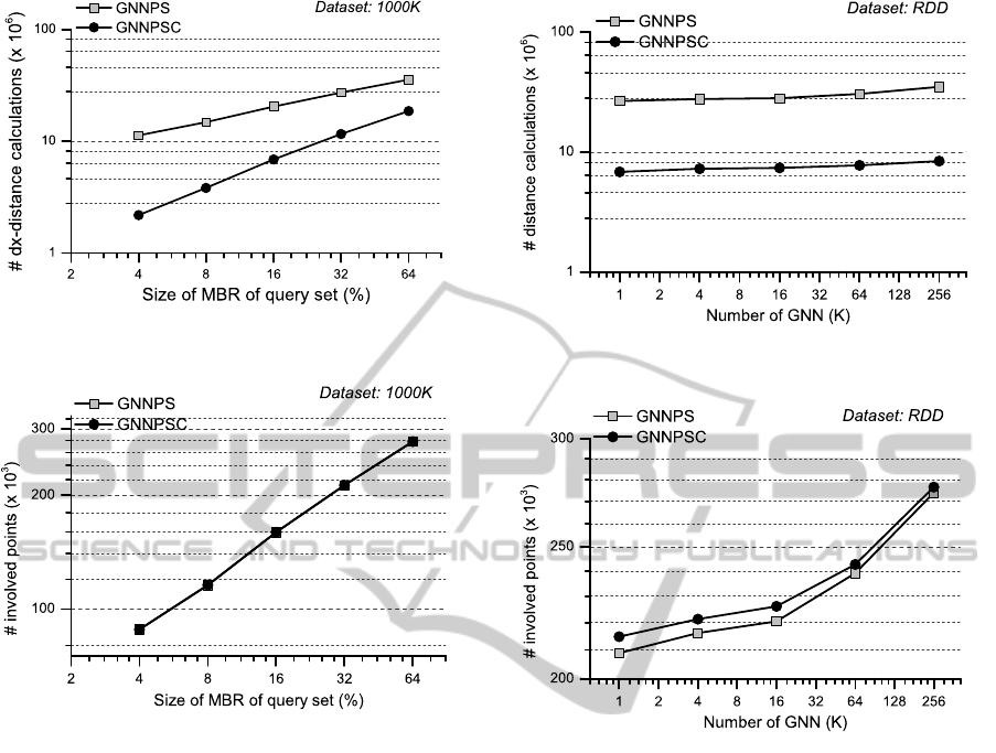
Figure 4: # dx-distance calculations of the algorithms as a

function of the size of MBR (1000K data set).

Figure 5: # Points involved in calculations of the algorithms

as a function of the size of MBR (1000K data set).

set MBR leads to an increase of the execution time,

but with a smaller rate of increase. The size of MBR

M was increased with a ratio of 4. The execution time,

dx-distance and complete distance (dist) calculations

was increased with ratio in the range 1.2 up to 2 for

all data sets of real and synthetic data. For the same

parameter settings and data set, in Figure 5, we de-

pict the effect of the size of the query-set MBR on

the number of points involved in calculations. We ob-

serve that this number of points is increased as M in-

creases with a ratio smaller than 1.4. We observe in

this ﬁgure that the number of points involved almost

identical and the two lines are overlapped.

In Figure 6, we depict the effect of the number

of group nearest-neighbors, K, on distance calcula-

tions of both algorithms for the RDD data set (the

number of query points, N, was equal to 128 and the

size of query-set MBR was 8% of the data set space).

Analogous diagrams created for execution times and

dx-distance calculations had similar appearance. It is

obvious that the increase of K does not signiﬁcantly

affect the execution time, dx-distance and complete

distance (dist) calculations. For the same parameter

Figure 6: # distance calculations of the algorithms as a func-

tion of K (RDD data set).

Figure 7: # Points involved in calculations of the algorithms

as a function of K (RDD data set).

settings and data set, in Figure 7, we depict the effect

of K on the number of points involved in calculations.

We observe that this number of points is increased so

slowly that it is going to be seen for values of K larger

than 64.

From the above experiments, we conclude that:

• The number of points of data sets (P) involved

in the calculations of both algorithms is almost

equal. However, the execution time for GNNPSC

remains always lower than the execution time of

GNNPS, due to the pruning condition and the

lower dx-distance calculations cost.

• The main advantages of the Plane-Sweep method

are the absence of recalculation, as each point is

used in calculations once at most, and the absence

of backtracking.

• The decrease of the number of points involved in

the calculations with respect to number of query

points can be justiﬁed when the MBR size is con-

stant.

Plane-SweepAlgorithmsfortheKGroupNearest-NeighborQuery

5 CONCLUSIONS AND FUTURE

WORK

Processing of GNNQs has been based on index struc-

tures, so far. In this paper, for the ﬁrst time, we

present new PS algorithms that can be efﬁciently ap-

plied on RAM-based data for processing the GNNQ.

As the experimentation that we performed, using syn-

thetic and real data sets, shows the use of median (in

GNNPS) and, even more, the use of median and cen-

troid (in GNNPSC), prunes the number of points in-

volved in processing and the number of calculations.

Although, in this paper, we do not present a com-

parison of our algorithms with respect to the algo-

rithms presented in (Papadias et al., 2004), compar-

ing the results that we have presented to the results of

(Papadias et al., 2004) for data sets of similar size (ap-

proximately 24.5K and 192/195K points) we observe

that our algorithms achieve competitive performance.

This is an initial observation. A detailed compari-

son could be performed in the future, using the same

data sets on the same machine. Moreover, the algo-

rithms we present could be transformed / extended to

work on high volume, disk resident data that are trans-

ferred in RAM in blocks. Moreover, the application

of Plane-Sweep to other spatial queries (like Reverse

NNQ) could lead to interesting techniques.

ACKNOWLEDGEMENTS

Work supported by the GENCENG project (SYN-

ERGASIA 2011 action, supported by the Euro-

pean Regional Development Fund and Greek Na-

tional Funds); project number 11SYN 8 1213. Work

also supported by the MINECO research project

[TIN2013-41576-R] and the Junta de Andaluc

ıa re-

search project [P10-TIC-6114].

REFERENCES

Ahn, H., Bae, S. W., and Son, W. (2013). Group nearest

neighbor queries in the L

plane. In TAMC Confer-

ence, pages 52–61. Springer.

Hashem, T., Kulik, L., and Zhang, R. (2010). Privacy

preserving group nearest neighbor queries. In EDBT

Conference, pages 489–500. ACM.

Hinrichs, K., Nievergelt, J., and Schorn, P. (1988). Plane-

sweep solves the closest pair problem elegantly. In-

formation Processing Letters, 26(5):255–261.

Jacox, E. H. and Samet, H. (2007). Spatial join techniques.

ACM Trans. Database Syst., 32(1):7.

Jiang, T., Gao, Y., Zhang, B., Liu, Q., and Chen, L.

(2013). Reverse top-k group nearest neighbor search.

In WAIM Conference, pages 429–439. Springer.

Li, H., Lu, H., Huang, B., and Huang, Z. (2005).

Two ellipse-based pruning methods for group near-

est neighbor queries. In ACM-GIS Conference, pages

192–199. ACM.

Li, J., Wang, B., Wang, G., and Bi, X. (2014). Efﬁcient pro-

cessing of probabilistic group nearest neighbor query

on uncertain data. In DASFAA Conference, pages 436–

450. Springer.

Lian, X. and Chen, L. (2008). Probabilistic group nearest

neighbor queries in uncertain databases. IEEE Trans.

Knowl. Data Eng., 20(6):809–824.

Luo, Y., Chen, H., Furuse, K., and Ohbo, N. (2007). Ef-

ﬁcient methods in ﬁnding aggregate nearest neighbor

by projection-based ﬁltering. In ICCSA Conference,

pages 821–833. Springer.

Namnandorj, S., Chen, H., Furuse, K., and Ohbo, N. (2008).

Efﬁcient bounds in ﬁnding aggregate nearest neigh-

bors. In DEXA Conference, pages 693–700. Springer.

Papadias, D., Shen, Q., Tao, Y., and Mouratidis, K. (2004).

Group nearest neighbor queries. In ICDE Conference,

pages 301–312. IEEE.

Papadias, D., Tao, Y., Mouratidis, K., and Hui, C. K.

(2005). Aggregate nearest neighbor queries in spatial

databases. ACM Trans. Database Syst., 30(2):529–

576.

Preparata, F. P. and Shamos, M. I. (1985). Computational

Geometry - An Introduction. Springer, New York, NY.

Rigaux, P., Scholl, M., and Voisard, A. (2002). Spatial

databases - with applications to GIS. Elsevier, San

Francisco, CA.

Roumelis, G., Vassilakopoulos, M., Corral, A., and

Manolopoulos, Y. (2014). A new plane-sweep algo-

rithm for the k-closest-pairs query. In SOFSEM Con-

ference, pages 478–490. Springer.

Zhang, D., Chan, C., and Tan, K. (2013). Nearest group

queries. In SSDBM Conference, page 7. ACM.

Zhu, L., Jing, Y., Sun, W., Mao, D., and Liu, P. (2010).

Voronoi-based aggregate nearest neighbor query pro-

cessing in road networks. In ACM-GIS Conference,

pages 518–521. ACM.

APPENDIX

Lemma: The sum of dx-distances between one given

point p(x,y) ∈ P and all points of the query set Q

(sumdx(p, Q)):

A Is minimized at the median point q[m] (where q[m]

is the array notation of q

B For all p.x ≥ q[m].x, sumdx is constant or increas-

ing with the increment of x, and

C For all p.x < q[m].x, sumdx is increasing while x

decreases.

GISTAM2015-1stInternationalConferenceonGeographicalInformationSystemsTheory,ApplicationsandManagement

k-1

m+1

M-1

k-1

m+1

M-1

// //

k΄-1

k -1΄

p΄

x x΄

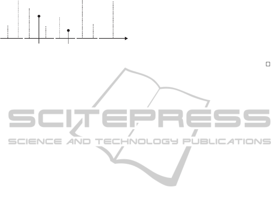
Figure 8: The point p has K query points on the left and the

point p

.x > p.x) has K

query points on the left.

Proof: Property A has been proved in (Ahn et al.,

2013). To prove property B, for every point p ∈ P

and q ∈ Q, we use

∆x(p, q) =



p.x − q.x if p.x ≥ q.x

q.x − p.x if p.x < q.x

If the point p has K query points on

the left (p.x < q[K − 1].x) and M − K

query points on the right (Figure 8), then:

sumdx(p,Q) =

K−1

∑

i=0

(p.x − q[i].x) +

M−1

∑

i=K

(q[i].x − p.x)

= K p.x −

K−1

∑

i=0

q[i].x +

M−1

∑

i=K

q[i] − (M − K)p.x

= (2K − M)p.x −

K−1

∑

i=0

q[i].x +

M−1

∑

i=K

q[i].x

For another point p

∈ P with p

.x > p.x which

has K

query points on the left (Figure 8)

and M − K

query points on the right, it is:

sumdx(p

,Q) = (2K

− M)p

.x −

−1

∑

i=0

q[i].x +

M−1

∑

i=K

q[i].x

The difference between dx-distances of the points p

and p is:

∆sumdx = sumdx(p

,Q) − sumdx(p, Q)

= (2K − M)(p

.x − p.x)

− K)p

.x −

−1

∑

i=K

q[i].x

If the set of the query points Q has cardinality M and

this is an even number then there are two medians

q[m1] and q[m2], while if M is odd then there is only

one median point q[m].

B.1 M is even and q[m1].x ≤ p.x < p

.x then

M ≤ 2K ≤ 2K

so (2K − M) ≥ 0, (p

.x − p.x) ≥ 0 and

− K)p

.x −

−1

∑

i=K

q[i].x ≥ 0

because p

.x ≥ q[i].x, whereas K ≤ i ≤ K

B.2 All of the above apply to M if it is odd and it

is only one median point q[m].x ≤ p.x < p

.x. It is

proven that for all points p on the right of the median

query point the sum of dx-distances is increasing.

C For both types of cardinality of the query set Q and

for the case p.x < p

.x < q[m].x it is:

∆sumdx = (2K − M)(p

.x − p.x) + 2(K

− K)p

−2

−1

∑

i=K

q[i].x

≤ (2K − M)(p

.x − p.x) + 2(K

− K)p

−2(K

− K)p.x

= 2(K − M)(p

.x − p.x)

+2(K

− K)(p

.x − p.x)

= (2K − M + 2K

− 2K)(p

.x − p.x)

= (2K

− M)(p

.x − p.x) < 0

It is proven that for all points p on the left of the

median query point the sum of dx-distances is strictly

decreasing.

Plane-SweepAlgorithmsfortheKGroupNearest-NeighborQuery