Optimizing Routine Maintenance Team Routes

Francesco Longo, Andrea Rocco Lotronto, Marco Scarpa and Antonio Puliaﬁto

Dipartimento DICIEAMA, Universit

a degli Studi di Messina,

Viale F. Stagno d’Alcontres, 31 - 98166 Messina (ME), Italy

Keywords:

Routine Maintenance Interventions, Metaheuristic Approaches, Simulated Annealing, Scheduling Problems,

Optimization Problems.

Abstract:

Simulated annealing is a metaheuristic approach for the solution of optimization problems inspired to the

controlled cooling of a material from a high temperature to a state in which internal defects of the crystals

are minimized. In this paper, we apply a simulated annealing approach to the scheduling of geographically

distributed routine maintenance interventions. Each intervention has to be assigned to a maintenance team and

the choice among the available teams and the order in which interventions are performed by each team are

based on team skills, cost of overtime work, and cost of transportation. We compare our solution algorithm

versus an exhaustive approach considering a real industrial use case and show several numerical results to

analyze the effect of the parameters of the simulated annealing on the accuracy of the solution and on the

execution time of the algorithm.

1 INTRODUCTION

The use of limited resources with utilization re-

quests over time originates a class of problems called

scheduling problems (W. Herroelen et al., 1999). The

contexts with this type of problems are multiple and,

consequently, for each of such contexts the ﬁnal ob-

jectives, the number and kind of the limited resources,

and the number and kind of the utilization requests

can be different. Moreover, the same problem could

not exhibit a unique solution. Instead, a set of solu-

tions that are all admissible can be generated, differ-

entiated by their cost. The nature of such a cost and

the way it is evaluated and determined is of course

different in different application contexts. However,

even if the application context changes, the follow-

ing property is usually satisﬁed: making a minimal

change to a particular solution of a scheduling prob-

lem can produce a substantial change in its cost. This

determines, in the general economy of any applica-

tion context, the necessity to ﬁnd a solution to a spe-

ciﬁc scheduling problem that is as less expensive as

possible. Moreover, it makes such a task particularly

difﬁcult given that small perturbations can heavily in-

ﬂuence the overall cost.

An algorithm exploited to solve this kind of prob-

lems usually tests if a given solution is admissible

for the problem and, deﬁning a cost function (usu-

ally depending on the aspects of the problem that is

necessary to minimize/maximize), calculates its cost.

Problems of this nature where the goal is to mini-

mize/maximize a cost function are generally identi-

ﬁed as optimization problems.

In this paper, we take into consideration the prob-

lem of scheduling a list of geographically distributed

routine maintenance interventions among a set of

maintenance teams, taking into account team skills,

cost of overtime work, and cost of transportation.

This kind of problems can present a set of admissible

solutions that is too large to implement an algorithm

that assesses all of them in order to determine the one

with the minimum cost, in a ﬁnite time. Therefore, we

follow a different approach exploiting a metaheuristic

technique (F. Glover and G. Kochenberger, 2003).

In particular, we exploit the simulated annealing

(SA) (Fleischer, 1995) metaheuristic to solve our rou-

tine maintenance scheduling problem with the goal of

optimizing the routes of the maintenance teams mini-

mizing the cost and trying to maximize the number of

maintenance operations actually performed in a given

day. In order to show the effectiveness of our ap-

proach, we take into consideration a real industrial

use case provided by Meridionale Impianti

, a com-

pany active in the industrial and electrical plant de-

sign sector. We compare the solution obtained by

http://www.merimp.com/en/

535

Longo F., Rocco Lotronto A., Scarpa M. and Puliaﬁto A..

Optimizing Routine Maintenance Team Routes.

DOI: 10.5220/0005400105350546

In Proceedings of the 17th International Conference on Enterprise Information Systems (ICEIS-2015), pages 535-546

ISBN: 978-989-758-096-3

 2015 SCITEPRESS (Science and Technology Publications, Lda.)

our approach with the exact solution obtained by ap-

plying an exhaustive algorithm that comprehensively

enumerates all the solutions ﬁnding the one that pro-

duces the minimal cost. We also perform a large set

of experiments evaluating the impact of the different

parameters of our SA approach to the accuracy of the

solution and the efﬁciency of the algorithm in terms

of execution time, with the aim of tuning the optimal

values of such parameters for future execution of the

same algorithm.

2 RELATED WORK

In this paper, we present an efﬁcient and general

method for solving routine maintenance scheduling

problems based on SA metaheuristic. Several works

in literature propose the use of SA for the solution

of scheduling problems in the context of the main-

tenance of speciﬁc installations, especially power

plants. In (J.T. Saraiva et al., 2011), authors address

the problem of the periodic maintenance of electric

generators by using SA. They aim at scheduling sys-

tem maintenance operations along a planning horizon

assuming that the time interval between maintenance

actions for the same generator is ﬁxed. In our ap-

proach, we do not take into consideration the time in-

terval between maintenance actions but we deal with

the scheduling of interventions that are supposed to

be conducted in a certain working day accordingly to

a predetermined business policy. As in (J.T. Saraiva

et al., 2011), (Keshav P. Dahal and Nopasit Chakpi-

tak, 2006) deals with the maintenance of generators

in a power plant by using a hybrid approach based

on a combination of genetic algorithms and SA. In

(Ibrahim El-Amin et al., 1999), the tabu search meta-

heuristic is applied to the maintenance of generators

in a power station with the aim of reducing the cost

associated with the management of the maintenance

operations and to increase the time interval between

two maintenance operations for the same generator.

In our case a pure SA approach is exploited mainly

focusing on the overall cost of performing a set of ge-

ographically distributed maintenance operations dur-

ing a working day taking into account transportation

and overtime costs.

More generally, the SA metaheuristic and its vari-

ations are often used for the solution of optimiza-

tion problems in several application ﬁelds spanning

from ICT to biomedicine. In (Chun-Cheng Lin et al.,

2014), SA, combined with additional momentum

terms in order to improve cooling rate, is exploited to

solve the problem of router node placement with ser-

vice priority constraint to improve the performance of

a wireless mesh network. In (Allen G. Brown et al.,

2014), the SA algorithm is adopted for creating ma-

neuver plans for the guidance of a satellite cluster. In

a gene expression data matrix, a bicluster is a subma-

trix of genes and condition. The problem of detecting

the most signiﬁcant bicluster has been shows to be

NP-Complete. In (Kenneth Bryan et al., 2006), the

authors present a biclustering technique based on SA

to efﬁciently discover the more signiﬁcant biclusters.

In this paper, we use SA to solve a maintenance

operation scheduling problem. During problem for-

malization we do not take into consideration any spe-

ciﬁc application context. However, we show its ap-

plication to a real industrial use case dealing with the

maintenance of energy plants. We are interested in

routine maintenance operations, i.e., maintenance op-

erations that are not related to an actual failure of the

considered system but are scheduled in advance. We

start from the assumptions that a set of maintenance

operations are scheduled to be conducted in a speciﬁc

day and our goal is to optimize the maintenance team

routes and maximize the number of interventions that

are actually performed. Contrary to maintenance op-

erations upon failures, such routine operations can be

postponed if it is not possible to guarantee that all

the operations that are supposed to be conducted in

a day will be actually fulﬁlled. However, our algo-

rithm is also able to deal with maintenance operations

that need to be executed with a higher priority.

3 REFERENCE SCENARIO

We take into consideration a company that needs to

perform maintenance operations in a set of geograph-

ically distributed locations. We only deal with routine

maintenance interventions, i.e., interventions that are

scheduled in advance. However, our approach also

takes into account that some higher priority interven-

tions could be necessary, representing failures and/or

speciﬁc situations that need immediate attention. We

focus on the set of maintenance operations that need

to be performed in a single day by a limited set of

maintenance resources. The maintenance resources

are represented by a number of teams, each composed

of a set of company employees and one vehicle. The

teams leave from the company principle headquarters

in the morning, follow a speciﬁc route established in

advance, perform all the maintenance interventions

that they have been assigned to, and return to their

starting point. This kind of problems falls under the

class of scheduling problems.

The problem we need to solve is to assign the

maintenance operations that are supposed to be con-

ICEIS2015-17thInternationalConferenceonEnterpriseInformationSystems

536

ducted in the considered day to the teams. Constraints

are present related to the nature of each maintenance

intervention. In fact, all maintenance operations have

speciﬁc characteristics in terms of both the location

where the intervention needs to be conducted and the

technical skills that are necessary to accomplish the

intervention. Being each intervention team composed

of one or more workers and one vehicle, accordingly

to the technical skills that each worker presents and

to the characteristics of the vehicle (that can reach a

speciﬁc location or not), it is possible to understand

which teams are able to perform a speciﬁc interven-

tion (it may be a subset of all the teams).

Of course, maintenance activities represent a cost

for the company. In our reference scenario, costs are

related to the hourly wage of the workers and to the

transportation expenses. A worker hourly wage in-

creases if the worker needs to do overtime, so a solu-

tion algorithm assigning interventions to teams needs

to minimize the possibility to go into overtime taking

into consideration both the time that is needed to per-

form each maintenance intervention and the traveling

time for a team to move from one intervention site to

the following. Transportation expenses are mainly re-

lated to fuel and maintenance for all the vehicles used

during the working day.

The main objective of this paper is to provide an

algorithm that automatically assigns the maintenance

interventions to the worker teams, taking into consid-

eration the above reported constraints with the aim of

minimizing the overall cost for the company.

4 PROBLEM FORMULATION

This section provides a formalization of the scenario

described in Section 3 unambiguously describing all

the characteristics of the considered scheduling prob-

lem, together with all the constraints and the costs that

need to be taken into account. Starting from our for-

malization, in Section 5, we will ﬁrst provide the so-

lution based on SA and then we will present an ex-

haustive algorithm that will be used as a reference for

the solution of the problem.

Let Q indicate the set of available maintenance

teams and let Q be the cardinality of such a set (Q =

|Q |), i.e., the total number of teams. Moreover, let

C indicate the set of all the possible technical skills

of the company workers, while C is the total number

of skills (C = |C|). We use I to indicate the set of

all the possible kinds of maintenance operations and

I to indicate their total number (I = |I|). Finally, let

P indicate the set of all the possible geographic loca-

tions for the maintenance interventions and let P be

the cardinality of such a set (P = |P |), i.e., the total

number of sites where maintenance operations can be

conducted.

Each day, a total number of L maintenance inter-

ventions need to be carried out by the Q teams. We

indicate with L the list of such interventions, with

L = |L|. Each maintenance intervention l ∈ L is char-

acterized by the following information:

• geographic location: the geographical coordinates

of the site p

∈ P where the maintenance interven-

tion l needs to be performed;

• maintenance operation: the maintenance opera-

tion i

∈ I that actually needs to be performed dur-

ing intervention l;

• execution time: the time t

∈ R that is necessary

to carry out the maintenance intervention l, once

on site;

• priority: the level of priority c

∈

{normal,urgent} assigned to intervention

The goal of the scheduling algorithm that we need

to design is to determine:

• the optimal number of maintenance interventions

that each team has to carry out (denoted with L

≤

L where 1 ≤ q ≤ Q);

• the actual list L

of maintenance operations each

team has to perform among those in L;

• the optimal order each team has to perform the

maintenance operations, i.e., the optimal ordering

of list L

;

Note that L

= |L

| and that the following constrains

apply:

∑

q=1

≤ L, (1)

[

q=1

⊆ L. (2)

Eq. (1) and (2) explicitly take into consideration the

possibility that, in the considered working day, not

all the scheduled maintenance interventions are actu-

ally performed (presence of ≤ and ⊆ symbols). This

could happen if an overtime is needed to exhaustively

perform all the maintenance operations for some of

the teams and if such a cost overcomes the cost asso-

ciated with the missing interventions.

If there are maintenance operations that require

speciﬁc skills, they necessarily have to be included

in the list of one of the teams whose components have

those skills. Let us deﬁne

: Q → 2

(3)

OptimizingRoutineMaintenanceTeamRoutes

537

associating to each maintenance team the set of skills

they possess, and

: I → 2

(4)

that associates to each speciﬁc maintenance opera-

tion the set of skills that are necessary to carry it out.

Then, a maintenance operation l ∈ L can be assigned

to team q ∈ Q if and only if F

(l) ⊆ F

(q).

Finally, if some of the maintenance interventions

in L exhibit a urgent priority they need to be included

in lists L

in the top positions. In the following, we

will indicate with L

[i].priority the priority assigned

to the i

intervention assigned to team q.

Let us denote the list of the geographical positions

and the execution times of the maintenance operations

assigned to team q as follows:



),(p

),... ,(p

)



where:

• p

∈ P is the position of the i

maintenance op-

eration assigned to team q;

• t

∈ R is the execution time of the i

maintenance

operation for team q;

with 1 ≤ i ≤ L

. In particular, let p

indicate the po-

sition of the location from where team q leaves at the

beginning of the working day and let p

indicate

the ﬁnal position to where the team has to go back.

Let v

deﬁne the travel time associated with the i

maintenance operation for the q team. Of course, v

depends on p

i−1

and p

and can be obtained by ap-

plying a routing algorithm ﬁnding the best route from

one geographical location to another. As an assump-

tion, v

is the travel time that is necessary for the

team to go back to the ﬁnal position.

For each team q to which a list of maintenance

operations L

has been assigned, the duration of the

working day D

can be computed as follows:

∑

i=1

) (5)

with t

= 0.

Denoting with D the maximum duration of the

working day, we want D

< D for each team. If it

is not possible to perform all the maintenance opera-

tions L in the working day, we deﬁne

L as the number

of maintenance operations that can be carried out dur-

ing the standard working hours. This

L operations are

associated with a normal cost, while we associate a

cost of overtime for the remaining maintenance oper-

ations. For each travel of each team, we associate a

cost CV

that can be computed as a function of the to-

tal distance associated with the i

maintenance opera-

tion of team q also including vehicles wear out. It can

be assumed that there is an additional cost for each

team whose duration of the working day exceeds D.

Therefore, if D

> D, this generates a cost of overtime

and we indicate it with CS

All this assumed, the multi-objective optimization

problem for our scenario can be formally deﬁned as

follows:

Problem 1:

Find L

(with 1 ≤ q ≤ Q) such that:

∑

q=1

∑

i=1

is minimized;

ii)

∑

q=1

is minimized;

iii)

L is maximized;

iv) ∀q,∀i : F

(i) ⊆ F

(q);

v) ∀q,∀i : L

[i].priority ≤ L

[i + 1].priority.

5 SOLUTION ALGORITHMS

5.1 Background on SA

Simulated annealing (SA) is commonly considered to

be the oldest meta-heuristic which explicitly applies

a strategy to avoid getting stuck in local minimum,

while searching the problem solution space (C. Blum

and A. Roli, 2003). The name and the inspiration of

SA derive from the physical phenomenon known as

annealing. The annealing process consists in ﬁrstly

heating a material to high temperature and then cool-

ing it in a controlled manner. This process increases

the size of the material crystals, while reducing their

internal defects.

The SA algorithm has been ﬁrstly introduced as

an adaptation of the Metropolis-Hasting algorithm, a

Montecarlo method to generate states of a thermody-

namic system (N. Metropolis et al., 1953). In such a

work, the SA algorithm produces a sequence of mate-

rial states:

...,s

i+1

i+2

,...,s

i+n−1

,....

Starting from the system initial state, the next state of

the sequence is generated by applying a perturbation

mechanism. Such a mechanism randomly produces a

new state which is close to the given one in terms of

their amount of thermodynamic energy. A sequence

of energy levels is then produced:

...,E

i+1

i+2

,...,E

i+n−1

,...

ICEIS2015-17thInternationalConferenceonEnterpriseInformationSystems

538

with the aim of reaching the system state with the

lower possible energy level. To this aim, as already

reported above, the SA exploits a strategy that seeks

to avoid local minimum.

At each algorithm iteration, starting from a state s

with energy E

, the SA algorithm randomly generates

a new state s

i+1

with energy E

i+1

. If the new state has

an amount of energy such that ∆E = (E

i+1

−E

) ≤ 0,

the new state is accepted as the current state, thus low-

ering the energy of the system. On the other hand,

if ∆E > 0, i.e., the energy of the system would be

increased, the algorithm accepts the new state, even

if it is worst than the previous one, accordingly to

a probabilistic approach that depends on the actual

temperature of the system. In fact, as in the physi-

cal annealing process, in the SA algorithm, starting

from a state with a high temperature, the temperature

is gradually lowered while advancing in the genera-

tion of new system states. When a newly generated

state produces a difference in energy greater than zero

(∆E > 0), the new state is accepted with a probabil-

ity equal to e

(−∆E/T )

, where T is the current temper-

ature (so called Metropolis criterion (N. Metropolis

et al., 1953)). This results in a high probability to ac-

cept new states, even if they are worst than the previ-

ous one, during the initial iterations of the algorithm.

However, while lowering the temperature also the ac-

ceptance probability will decrease. This strategy al-

lows SA not to get stuck in local minimum.

Applying the SA meta-heuristic to a given opti-

mization problem involves designing all its character-

istic aspects adapting them to the speciﬁc context (D.

T. Pham and D. Karaboga, 2000) as detailed in the

following.

Solutions Space. The solution space S represents the

set of all the possible solutions to the given problem

that the SA approach has to be able to generate. Tak-

ing into consideration the above reported discussion,

it represents all the possible states s

that the system

can assume.

Cost Function. In optimization problems, deﬁning a

cost function that is used as the objective function to

minimize is needed. In the SA annealing metaphor,

the cost function of the optimization problem is asso-

ciated with a function f determining, for each system

state, the value of the associated energy:

= f (s

). (6)

Generation Mechanism of the Neighboring Solu-

tions. When using SA for the solution of a problem,

it is necessary to formally deﬁne a mechanism that,

given the current solution, allows to generate a new

neighboring solution. In the SA metaphor, it is neces-

sary to deﬁne a function Ψ determining a new system

state s

i+1

from current state s

i+1

= Ψ(s

). (7)

Of course, while designing such a function, it is nec-

essary to take into consideration a criteria that allows

to determine if a new solution is near to the current

one. This is strictly related to the nature of the given

optimization problem.

Cooling Scheme. The way cooling is performed in

SA is characterized by four aspects: i) initial temper-

ature; ii) temperature updating mechanism; iii) num-

ber of iterations for each temperature value; iv) stop

criterion. Also in the case of the solution of an opti-

mization problem, it is necessary to design a speciﬁc

cooling scheme that allows to reach a good solution,

while still containing execution time.

Acceptance Rule. A newly generated solution need

to be accepted or discarded accordingly to a certain

criterion. In SA, to accept or discard a newly gener-

ated state, Metropolis criterion or one of its variations

are often used. Such criteria are usually exploited also

in the case of the solution of an optimization problem.

5.2 Formalization of a Solution

In order to show how SA has been exploited for

the solution of our optimization problem, namely the

problem of scheduling a list of geographically dis-

tributed routine maintenance interventions among a

set of maintenance teams, taking into account team

skills, cost of overtime work, and cost of transport,

it is ﬁrst necessary to deﬁne how a possible problem

solution can be represented in a formal way.

With this aim, let us consider a speciﬁc case in

which L = 10 maintenance interventions need to be

scheduled among Q = 4 maintenance teams. A pos-

sible solution of such a problem consists in ﬁnd-

ing the four lists L

, L

, and L

associating to

each team the interventions to perform in a speciﬁc

order. An example is the following: L

= {1,8},

= {2, 9,10}, L

= {4, 3}, L

= {7, 6,5}, i.e., the

ﬁrst team is scheduled to perform interventions num-

ber 1 and 8 in this order, the second team is scheduled

to perform interventions number 2, 9, and 10 in this

order, and so on. Such a problem solution can be for-

mally represented in a matrix form as follows:







1 0 0 0 0 0 0 2 0 0

0 1 0 0 0 0 0 0 2 3

0 0 2 1 0 0 0 0 0 0

0 0 0 0 3 2 1 0 0 0







. (8)

In such a matrix each row is associated with a main-

tenance team while each column refers to a mainte-

nance intervention. The values of nonzero elements

OptimizingRoutineMaintenanceTeamRoutes

539

indicates the order in which each intervention is per-

formed by the corresponding team. So, for exam-

ple, the element belonging to the ﬁrst row and to

the eight

column is equal to 2 because intervention

number 8 is scheduled to be performed by the ﬁrst

team as the second intervention in its list.

Generalizing such an example, a generic solution

of a generic instance of our scheduling problem is

given by a speciﬁc distribution of L maintenance in-

terventions among Q maintenance teams. Thus, if we

want to formally represent it in a matrix form, we

need a Q × L matrix A = {a

i, j

} such that i ∈ [1, Q],

j ∈ [1,L], and a

i, j

∈ [1,L]:

A =







1,1

1,2

·· · a

1,L

Q,1

Q,2

·· · a

Q,L







. (9)

In particular, being L the interventions to be per-

formed, the matrix in eq. (9) represents a solution

of our optimization problem only if a maximum of

L among its Q · L elements are nonzero:

nz(A) ≤ L (10)

where nz : R × R → N is a function that provides the

number of nonzero elements in a given matrix. More-

over, given that each matrix column is associated with

a speciﬁc intervention and given that each interven-

tion can be assigned only to one team, it follows that

in each column of matrix A only one element can be

nonzero, indicating the team to which the correspond-

ing intervention is assigned. Thus, indicating with c

the j

column of matrix A with j ∈ [1,L] (it is con-

sidered as a Q × 1 matrix):







1,1

2,1

Q,1













1,2

2,2

Q,2







,··· ,c







1,L

2,L

Q,L







(11)

then:

nz(c

) ≤ 1, ∀ j ∈ [1, L]. (12)

The use of symbol ≤ in both eq. (10) and (12) is due to

the fact that some interventions may not be scheduled

due to overtime cost.

Finally, the value of the nonzero element of each

column c

has to represent the execution order of the

maintenance intervention j ∈ [1,L] within the list of

interventions associated with the corresponding team.

In formula:

x, j

6= 0 ⇔ L

[(a

x, j

)] = j (13)

with x ∈ [1,Q] and j ∈ [1,L] and x is the index as-

sociated with the team to which the intervention j is

assigned.

Summarizing, a possible solution of our optimiza-

tion problem can be formally represented as the ma-

trix in eq. (9) subject to the structural constraints re-

ported in eq. (10), (12), and (13). Moreover, Problem

1 constraints iv) and v) should also be checked in or-

der to verify that the solution represented by a given

matrix is admissible for the given problem.

5.3 Applying SA to our Optimization

Problem

SA is a meta-heuristic for general applications.

Therefore, as already mentioned in Section 5.1, it is

necessary to design all its characteristic aspects adapt-

ing them to the speciﬁc context. In the case of our op-

timization problem, such aspects have been designed

as follows.

Solution Space. Accordingly to what reported in

Section 5.2, the solution space of our optimization

problem can be formally represented as the set of all

the possible Q × L matrices in the form of eq. (9):

S = {A

} (14)

with Q and L depending on the speciﬁc problem and

satisfying eq. (10), (12), and (13), and Problem 1 con-

straints iv) and v).

Cost Function. In our optimization problem, the cost

function associates a cost to each possible matrix in

S. Accordingly to the deﬁnition of Problem 1 and to

what has been exposed in Section 4, our cost function

is the following:

= f (A) =

∑

q=1

∑

j=1

∑

q=1

. (15)

Generation Mechanism of the Neighboring Solu-

tions. In our optimization problem, function Ψ :

S × {row,column} → S operates on a matrix in S re-

turning another matrix that is close to the ﬁrst one in

terms of disposal of its elements:

i+1

= Ψ(A

, p) (16)

with A

i+1

∈ S, p ∈ {row, column}.

The parameter p is used to deﬁne two ways of

modifying matrix A

in terms of element disposal ob-

taining matrix A

i+1

. In particular:

• Row Swapping. If p = row, two elements in a

row of the matrix are swapped. Speciﬁcally, we

randomly select one of the matrix rows in which

two or more nonzero elements are present, i.e., we

randomly select a team whose list of interventions

contains two or more interventions:

generate q ∈ [1, Q] : |L

| > 1.

ICEIS2015-17thInternationalConferenceonEnterpriseInformationSystems

540

Then, we randomly select two different nonzero

elements in the row:

generate x, y ∈ [1, L] : a

q,x

6= a

q,y

6= 0

and we swap them, i.e., we invert the order in

which two interventions in the list are performed:

i+1

q,x

= a

q,y

, (17)

i+1

q,y

= a

q,x

• Column Swapping. If p = column, the nonzero

element of a column of the matrix is moved from

one row to another one, possibly modifying its

value if necessary. In particular, we randomly

select one of the matrix columns c

in which a

nonzero element is present, i.e., we select an in-

tervention l that is already assigned to a team:

generate l ∈ [1,L] : nz(c

) 6= 0, i.e., l ∈

[

q=1

Then, we randomly select one matrix row z in

which the corresponding element a

z,l

of the ma-

trix column c

is equal to zero:

generate z ∈ [1, Q] : a

z,l

= 0.

The value of the nonzero element in the column

vector c

is set to zero. Finally, if all the elements

of the row z in matrix A

are zero then element

i+1

z,l

in matrix A

i+1

is set to 1:

i+1

z,l

= 1 (18)

while, if in the row z in matrix A

there are

nonzero elements, we compute the maximum

value among all the elements in the row and we

assign to element a

i+1

z,l

in matrix A

i+1

the value:

i+1

z,l

= max(z,A

) + 1, (19)

i.e., we take one intervention from one team and

we give it to another one that will perform it as its

last intervention.

Cooling Scheme. The aspects of the cooling scheme

have been designed as follows:

• (a) initial temperature - An initial problem solu-

tion A

is generated and the initial temperature is

set to its cost:

T = E

(20)

• (b) temperature updating mechanism - We de-

signed an updating mechanism based on a cooling

factor α ∈ R

such that:

T = T − (α · T ) (21)

• (c) number of iterations for each temperature

value - n

∈ N iterations are performed for each

temperature value T by correspondingly generat-

ing n

solutions though the use of eq. (16):

,··· ,A

• (d) stop criterion - We designed a criterion which

is based on both the value of the temperature and

the progress of the SA algorithm itself. We de-

ﬁned a target temperature T

low

∈ [0, T [ at which

the SA algorithm is terminated. Moreover, we use

a vector vectE to store the cost associated with the

last |vectE| solutions:

vectE = {E

y+1

,··· ,E

y+|vectE |

} (22)

If the cost associated with such solutions is ex-

actly the same for a number of temperature levels

equal to |vectE| the algorithm is terminated:

(Q,L)

= E

y+1

(Q,L)

= ·· · = E

y+|vectE |

(Q,L)

(23)

Acceptance Rule. The solutions generated for each

temperature value T are compared using Metropolis

criterion. When solution A

i+1

is generated its cost

is computed by eq. (15) and the cost variation with

respect to solution A

is computed:

∆E = f (A

i+1

) − f (A

). (24)

If ∆E ≤ 0 the new solution is accepted. Otherwise, if

∆E > 0 the new solution is accepted only if

ξ < e

(−∆E/T )

(25)

where ξ is a random number uniformly distributed

over [0,1] and T is the current temperature. If ξ >

(−∆E/T )

the new solution is discarded and current

solution A

is used to generate a new one through

eq. (16).

Algorithm 1 reports all the steps of the SA algo-

rithm as applied to our routine maintenance problem.

Speciﬁcally, in lines 1-7 all the necessary vari-

ables are declared: s and s

represent the current solu-

tion and the neighboring solution, respectively; vec-

tor vectE of size d stores the cost of the last d solu-

tions; α is the cooling factor; T contains the initial

temperature of the system and the following tempera-

ture values while T

low

is the minimum temperature to

be reached; E and E

represent the cost of the current

solution s and of the neighboring solution s

, respec-

tively; n

is the number of iterations to be performed

for each temperature value. In line 9 the initial solu-

tion is generated through generate initial solution()

and in line 10 f () returns its cost (see eq. (6)). Such a

cost is used to set the temperature initial value in line

11. The SA algorithm itself consists of two nested

OptimizingRoutineMaintenanceTeamRoutes

541

Algorithm 1: SA algorithm for the solution of the routine

maintenance problem.

1: declare s, s

;

2: declare d;

3: declare α;

4: declare vectE[d];

5: declare T , T

low

;

6: declare E, E

;

7: declare n

;

9: s ← generate initial solution()

10: E ← f (s);

11: T ← E;

12: while T > T

low

13: i ← 1;

14: while i < n

15: s

← Ψ(s);

16: E

← f (s

);

17: ξ ← rand();

18: if E

≤ E or e

−(E

−E)/T

> r then

19: s ← s

;

20: E ← E

;

21: end if

22: i ← i + 1;

23: end while

24: vectE ← store last cost(vectE, E);

25: if check stop criteria(vectE,d) then

26: break;

27: end if

28: T ← T − (α · T );

29: end while

30: return s, E;

loops. The outer loop (lines 12-29) is used for tem-

perature cooling while the inner loop (lines 14-23)

is used to perform the n

iterations for each temper-

ature value. In particular, in lines 24-27 functions

store last cost() and check stop criteria() are used

to check if the last |vectE| = d solutions are exactly

the same. In such a case the algorithm is stopped.

Otherwise the algorithm stops as soon as temperature

low

is reached. In both cases, the current solution and

its cost are returned (line 30).

5.4 Exhaustive Algorithm

Through the use of the SA, we are not guaranteed that

the found solution is the best solution for our opti-

mization problem. It is therefore necessary to identify

a reference value to evaluate the quality of the solu-

tions found with the SA. To this purpose, we designed

an exhaustive algorithm.

Exhaustive algorithm is composed of two parts.

The ﬁrst part has the role to ﬁnd all the possible dis-

tributions of the L maintenance interventions to the Q

maintenance teams. The distribution operation sim-

ply executes the division of the L maintenance inter-

ventions to the Q maintenance teams by creating Q

unordered lists identiﬁed as U

[

q=1

⊆ L (26)

Where U

= |U

| : U

≤ L and U

[i] ∈ [1,Q] : i ∈

[1,L]. To solve the distribution operation a method

which use a vector with dimension L has been devel-

oped:

= {v

,··· v

} (27)

Each elements of the V

vector represents one of the

maintenance interventions of the list L:

∈ L (28)

The value of each element of the vector V

determines

at which U

unordered list is assigned, whereas the

position in the vector determines the identiﬁer of the

maintenance operation:

[x] = i : x ∈ [1,L] (29)

The V

vector allows us to implement and automate

the generation of all the possible distributions of the L

maintenance operations to the Q maintenance teams,

using the V

vector like a number in Q basis with L

digits, it is possible to generate all the numbers in Q

in the range [0,Q

] by deﬁning the following function

= next(V

i−1

,b) (30)

where i ∈ [0, Q

] and V

= {0}. The function (30) re-

ceives in input a number V

i−1

expressed in array form

(27), and its basis b. Therefore the function generates

the next number of the input in basis b. This last num-

ber is always expressed in array form (27).

The second part of the exhaustive algorithm, us-

ing all vector form numbers found with function (30),

computes all the possible solutions for our problem

which are later evaluated to determine the best solu-

tion.

For each vector numbers all possible simple per-

mutations of the U

are evaluated. Therefore, for

each U

several solutions are generated for our prob-

lem, each evaluated to determine the best solution.

6 EXPERIMENTAL RESULTS

The use case, where the SA algorithm was applied, is

related to a real Italian company, located in the north

west of Sicily, with the responsibility of managing

the maintenance related to electrical installations. As

mentioned in Section 1 to perform the maintenance

operations the company needs to solve a scheduling

problem to minimize the overall cost for maintenance.

ICEIS2015-17thInternationalConferenceonEnterpriseInformationSystems

542

The solution of the optimization problem must be

found respecting the formalization of the objectives

and constraints speciﬁed in Problem 1.

In particular, the use case is related to a typical

working day, where the company needs to schedule

the daily maintenance operations to its maintenance

teams. The maintenance operations, occur in the elec-

trical installations managed by the company. The ge-

ographical points of installations and company head-

quarters compose the all possible geographical loca-

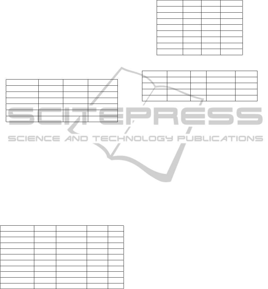
tions P deﬁned in Section 4 and listed in Table 1.

Table 1: Geographical points of installations.

Installation ID Latitude Longitude Name

1 38.000000 13.283333 Kaggio (A)

2 38.083333 13.500000 Bagheria (B)

3 38.050000 13.000000 Balestrate (C)

4 38.150000 13.083333 Terrasini (D)

5 38.033333 13.450000 Misilmeri (E)

6 38.116667 13.366667 Company (F)

As introduced in Section 4, L maintenance ser-

vices are provided in a typical working day; each of

them is characterized by an execution time, a set of

skills needed to perform the maintenance and a loca-

tion. We applied our optimization algorithm to the

L = 10 maintenance services of the referred company

reported in Table 2, where the maintenance services

are identiﬁed by an ID and the location where the

maintenance has to be done is identiﬁed by the same

ID used in Table 1 (Installation ID). In order to main-

tain the scenario as simple as possible, we assume that

all the maintenance intervention have the same prior-

ity.

Table 2: Maintenance interventions.

Interventions ID Duration Installation ID Skills ID Skills

1 120 1 1 {3}

2 180 2 2 {1,2}

3 120 2 1 {3}

4 90 3 3 {1}

5 180 3 2 {1,2}

6 60 5 4 {2}

7 120 4 2 {1,2}

8 120 1 5 {2,3}

9 180 5 6 {1,3}

10 120 4 5 {2,3}

The company has four maintenance teams (Q =

4), composed of one or more workers and a single

vehicle. These teams are the elements of Q . Each

worker has one or more skills, collected in C . In

our use case three possible skills have been identiﬁed

(C = 3) and they have been associated to each worker

as described in Table 3, where the cost per hour and

the maintenance team have been speciﬁed.

The vehicles owned by the company are summa-

rized in Table 4 together with the fuel type (petrol or

Table 3: Workers cost per hour and skills.

Worker ID Cost/h Skills Team ID

1 6.80 {1,2,3} 1

2 6.50 {1,2,3} 1

3 7.00 {1,2,3} 2

4 6.40 {1,2} 2

5 6.25 {1,2,3} 3

6 6.90 {3} 3

7 6.20 {1,2,3} 4

8 6.00 {3} 4

Table 4: Vehicles characteristics.

Vehicle ID Fuel type l/Km Wear/Km($) Team ID

1 Diesel 8.2 0.57 1

2 Diesel 8.2 0.57 2

3 Petrol 5.9 0.25 3

4 Petrol 5.9 0.25 4

diesel), the costs, and the maintenance team ID which

are assigned to.

Each maintenance team is characterized by both

the skills of its workers and the characteristics of its

vehicle. This means that each teams can perform only

the maintenance services ﬁtting adequate skills spec-

iﬁed through eq. (3) and (4). In the speciﬁc case of

the use case here considered, columns Skills ID and

Skills of Table 2 represents the function of eq. (4).

It is easy to see that the monetary cost of each team

depends on the workers hourly cost (Table 3) and on

the travel cost (Table 4).

To completely deﬁne the optimization problem,

we have to deﬁne the cost functions introduced in

Problem 1 (items i) and ii)). These functions depends

on the working day duration D, that is assumed to be

eight hours long (D = 8) in our use case. Let C

the hourly cost by each maintenance team during the

regular working time, C

is calculated by adding the

hourly wage of each worker of the team shown in Ta-

ble 3. In ii) is deﬁned the cost function to be applied

after the ﬁrst eight working hours. The cost CS

de-

ﬁned in Problem 1, representing the cost during the

extra working time, is deﬁend as CS

= 2 ∗ C

. The

cost CV

is computed using the data in Table 4 and

ﬁxed values for diesel and petrol cost that are 1.746

for the petrol and 1.627 for the diesel.

In the following, we will present the results ob-

tained by applying the optimization Algorithm 1 to

the problem deﬁned above. Since the SA is a based

on a meta-heuristic approach, we compare the results

with the real optimum solution computed through the

exhaustive algorithm (Section 5.4). The purpose of

the comparison is twofold: 1) evaluate the quality of

the solution, and 2) evaluate the time efﬁciency of the

algorithm. During our experiments, we varied the SA

parameters in order to show their impact on the ﬁnal

OptimizingRoutineMaintenanceTeamRoutes

543

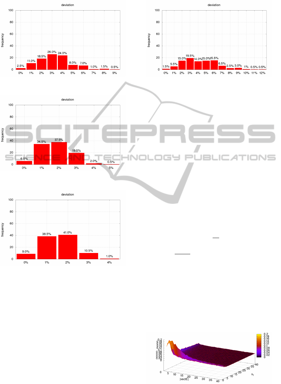
Figure 1: α = 0.3, n

= 30, T

low

= T − (T ∗ 0.999),

|vectE| = 20.

Figure 2: α = 0.03, n

= 30, T

low

= T − (T ∗ 0.999),

|vectE| = 20.

Figure 3: α = 0.003, n

= 30, T

low

= T − (T ∗ 0.999),

|vectE| = 20.

solution. We considered the parameters related to the

cooling (21) and to the stop criterion (23), speciﬁcally

α and n

for the cooling scheme, T

low

and |vectE| for

the stop criterion.

Given a set of ﬁxed parameters, we run the SA

algorithm 200 times and we computed the distance

of each obtained optimal solution with respect to that

evaluated by the exhaustive algorithm. The overall re-

sults are synthesized in Figures 1, 2 and 3 by varying

the α and with ﬁxed n

and T

low

; each histogram de-

picts the distribution of the deviations. As an example

Figure 1 shows that the Algorithm 1 has a probabil-

ity equal to 26% to give an estimation of the optimum

with an error equal to 3%. The graphs show that de-

Figure 4: α = 0.003, n

= 30, T

low

= T − (T ∗ 0.990),

|vectE| = 20.

creasing the value of α the accuracy of the result de-

creases accordingly, ranging from an an average devi-

ation of 3.275% with α = 0.3 to an average deviation

of 1.56% with α = 0.003.

Another set of experiments has been performed by

ﬁxing the value of α to 0.003 and varying the param-

eter T

low

from T

low

= T − (T ∗ 0.999) (Figure 3) to

low

= T − (T ∗ 0.990) (Figure 4), thus increasing the

value of the target temperate. This change produces a

sharp deterioration of the solutions found with Algo-

rithm 1 to an average deviation of 4.319 in Figure 4.

This deterioration is justiﬁed by the fact that fewer it-

erations are performed with Algorithm 1 to search the

solution of the optimization problem.

To evaluate how the parameters n

and |vectE| af-

fect the Algorithm 1 in the search of the solution, we

considered as a quality index the relative error E

the solution obtained by the exhaustive algorithm:

(31)

where E

−V

is the mean absolute error affect-

ing the solution, V

is the result of exhaustive algo-

rithm, and x

is the average value of the solutions ob-

tained from Algorithm 1. Figure 5 depicts E

versus

both n

and |vectE|. As can be seen in Figure 5, E

decreases when n

and |vectE| increase starting from

0 but its value does not substantially change when n

and |vectE| reach a certain threshold.

To better analyze the behavior of the SA algo-

rithm, we also considered the execution time, other

than the quality of the result, through the following

Figure 5: E

with α = 0.003 and T

low

= T − (T ∗ 0.999).

ICEIS2015-17thInternationalConferenceonEnterpriseInformationSystems

544

function:

,τ) = 1−



β ·

− min

∆





γ ·

τ − min

∆



(32)

The quantities used to deﬁne F

() are the following:

∆

= max

− min

, where max

and min

are the

maximum and the minimum relative error obtained by

varying n

and |vectE|; τ is the measured execution

time of the Algorithm 1; ∆τ = max

− min

, where

max

and min

are the maximum and the minimum

execution time obtained by varying the parameters n

and |vectE|; the parameters β and γ, such that β + γ =

1, are two constants used to give a different weight to

the quality of the solutions and to the execution time

of the Algorithm 1 respectively.

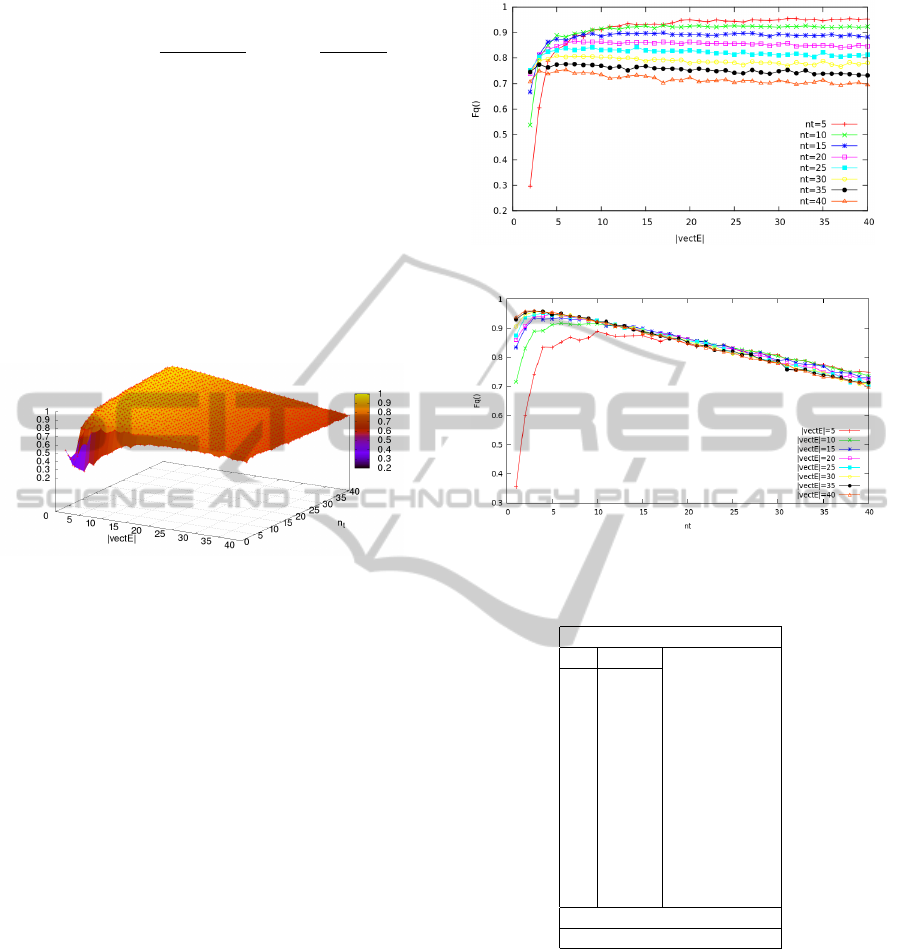
Figure 6: F

,τ) with β = 0.7 and γ = 0.3.

The graph in Figure 6 shows the trend of function

(32) computed with α and T

low

set to the optimal val-

ues found in the ﬁrst set of experiments (α = 0.003

and T

low

= T − (T · 0.999)) and by varying n

and

|vectE|. The values of β and γ are ﬁxed to β = 0.7

and γ = 0.3 in order to give more weight to the solu-

tion quality than to the execution speed of the Algo-

rithm 1. The analysis of the graph reveals a maximum

identifying the best pairs of parameters to optimize

the behavior with respect either the precision and the

execution time.

To better identify the value of the parameters, we

depicted in Figures 7 and 8 the 2-D versions of the

graph in Figure (6). In Figure 7, each line corresponds

to a single value of n

(z axis in Figure 6) whereas in

Figure 8 each line corresponds to a single value of

|vectE| (x axis in Figure 6).

Parameters n

and |vectE| carry out a comple-

mentary role. Using hight values of |vectE|, we im-

pose a stop criterion heavily based on temperature T ;

this conﬁguration produces excellent results as long

as n

doesn’t excessively increase otherwise a perfor-

mances degradation is manifested. As well shown in

Figure 8, the graph has a maximum located around

= 5 and |vectE| = 35.

As ﬁnal experimental results, we reported in Ta-

ble 5 the execution times obtained by running Algo-

rithm 1 with different sets of parameters and the exe-

Figure 7: F

,τ) with β = 0.7 and γ = 0.3.

Figure 8: F

,τ) with β = 0.7 and γ = 0.3.

Table 5: Execution Time Algorithm 1 and Exhaustive Al-

gorithm.

Execution Time Algorithm 1 (ms)

|vectE|

5 5 485.0

5 20 639.4

5 35 697.4

10 5 1057.2

10 20 1313.8

10 35 1442.4

20 5 2332.0

20 20 2746.4

20 35 2977.2

35 5 4304.8

35 20 4986.2

35 35 5259.0

Execution Time Algorithm 2 (ms)

2100000

cution time of the exhaustive algorithm. As can be ob-

served, Algorithm 1 completes in some milliseconds,

irrespective of the set of parameters, whereas the ex-

haustive algorithm needs a lot of minutes to ﬁnd the

ﬁnal problem solution.

7 CONCLUSIONS AND FUTURE

WORK

In this paper, we proposed the use of simulated an-

nealing for the solution of the scheduling problem of a

OptimizingRoutineMaintenanceTeamRoutes

545

set of geographically distributed routine maintenance

interventions. We based the choice of which team to

pick among the available ones for each intervention

and the order in which each team performs its inter-

ventions on several parameters, i.e., team skills, cost

of overtime work, and cost of transportation. We ap-

plied the proposed algorithm to a real industrial use

case provided by an electrical plant design company

and we compared it versus an exhaustive approach.

Several numerical results have been shown highlight-

ing the effects of the parameters of the simulated an-

nealing on the accuracy of the solution and on the ex-

ecution time of the algorithm. Future work will be

focused on implementing a complete tool for mainte-

nance intervention scheduling, testing and stressing

it on the ground of realistic use cases. Moreover,

we plan to combine the proposed approach with ad-

vanced routing algorithms analyzing the inﬂuence of

their efﬁciency on our solution technique.

ACKNOWLEDGEMENT

The research leading to these results has re-

ceived funding from the Italian National project

“SIGMA - Integrated Cloud-Sensor System for Ad-

vanced Multirisk Management” under grant agree-

ment PON01 00683.

REFERENCES

Allen G. Brown, Dr. Matthew, C. Ruschmann, Dr. Brenton

Duffy, Lucas Ward, Dr. Sun Hur-Diaz, Eric Ferguson,

and Shaun M. Stewart (2014). Simulated annealing

maneuver planner for cluster ﬂight. In 24th Interna-

tional Symposium on Space Flight Dynamics, Laurel,

MD, April 2014.

C. Blum and A. Roli (2003). Metaheuristics in combinato-

rial optimization: overview and conceptual compari-

son. In ACM Computing Surveys, Vol. 35, No. 3.

Chun-Cheng Lin, Lei Shu, and Der-Jiunn Deng (2014).

Router node placement with service priority in wire-

less mesh networks using simulated annealing with

momentum terms. In Systems Journal, IEEE (Vol-

ume:PP , Issue: 99 ).

D. T. Pham and D. Karaboga (2000). Intelligent optimisa-

tion techniques: genetic algorithms, tabu search, sim-

ulated annealing and neural networks. In Springer.

F. Glover and G. Kochenberger (2003). Handbook of meta-

heuristics. massachusetts. In Eds. New York: Kluwer

Academic Publish-ers.

Fleischer, M. (1995). Simulated annealing: past, present

and future. In Proceedings of the 1995 Winter Simu-

lation Conference, C. Alexopoulos, K. Kang, W. Lileg-

don, and G. Goldsman, Eds. 155161.

Ibrahim El-Amin, Salih Duffuaa, and Mohammed Abbas

(1999). A tabu search algorithm for maintenance

scheduling of generating units. In Electric Power Sys-

tems Research 54 (2000) 9199.

J.T. Saraiva, M.L. Pereira, V.T. Mendes, and J.C. Sousa

(2011). A simulated annealing based approach to

solve the generator maintenance scheduling prob-

lem. In Electric Power Systems Research 81 (2011)

12831291.

Kenneth Bryan, Padraig Cunningham, and Nadia Bol-

shakova (2006). Application of simulated annealing to

the biclustering of gene expression data. In Informa-

tion Technology in Biomedicine, IEEE Transactions

on (Volume:10 , Issue: 3 ).

Keshav P. Dahal and Nopasit Chakpitak (2006). Genera-

tor maintenance scheduling in power systems using

metaheuristic-based hybrid approaches. In Electric

Power Systems Research 77 (2007) 771779.

N. Metropolis, A. W. Rosenbluth, M.N. Rosenbluth, A.H.

Teller, and E. Teller (1953). Equation of state cal-

culations by fast computing machines. In Journal of

Chemical Physics, vol. 21, no. 6, pp. 10871092.

W. Herroelen, E. Demeulemeester, and B. De Reyck

(1999). Metaheuristics in combinatorial optimization:

overview and conceptual comparison. In J. Weglarz

(Ed.), Project Scheduling: Recent Models, Algorithms

and Applications, Kluwer Academic Publishers, pp.

126.

ICEIS2015-17thInternationalConferenceonEnterpriseInformationSystems

546