
Monoscopic Automotive Ego-motion Estimation and Cyclist Tracking
Johannes Gr
¨
ater and Martin Lauer
Institute of Measurement and Control, Karlsruhe Insitute of Technology, Karlsruhe, Germany
1 RESEARCH PROBLEM
In traffic accidents cyclists are always counted as a
vulnerable group suffering from heavy injuries and
fatalities. A particularly dangerous type of collision
involves trucks that turn to the right without recogniz-
ing cyclists driving on their lane in a blind spot. Even
though it is not the most frequent type of accident the
chance of survival for a cyclist involved is low.
One of the main causes for the collision is that the
truck drivers only have a limited field of vision. The
cyclists in the surroundings are hard to perceive due
to their smaller size. Besides, it is difficult to pre-
dict their behavior. The velocity of a cyclist is usu-
ally comparable to a slowly running car and they must
share the same road with other traffic participants,
which makes them easy to be occluded by other ve-
hicles. Hence, this reduces the truck driver’s reaction
time once they are noticed. This also explains that the
heaviest accidents involving trucks and cyclists often
happen when a truck turns right at an intersection.
In order to solve this problem on an intelligent
level we are aiming at developing a driving assistance
system for trucks to avoid possible accidents with cy-
clists. The main task is to detect the cyclists with the
help of a state-of-the-art hardware setup consisting of
a single-row Light Detection And Ranging(LIDAR)-
Sensor in combination with a camera. Based on the
detection, the movement of the cyclist is estimated
and its behavior is predicted so that the risk of ac-
cidents can be assessed. An intelligent warning strat-
egy alarms the truck driver in dangerous situations to
avoid accidents.
The aim of this work is to estimate the metric tra-
jectory of the ego-vehicle and the cyclist using a sin-
gle camera and a low-cost single-row laser scanner.
For estimating the ego-motion without scale we com-
plement existing methods to satisfy the requirements
of our application. The main challenge of mono-
scopic Visual Odometry is the unobservability of the
scale of the scene. The focus of this project lies on
estimating the scale from scene implicit information
combined with a priori knowledge about the scenery.
On the other hand external sensors are applied to ob-
tain more data about the scale and find an optimal con-
figuration for estimating a scaled trajectory of a car in
various environments.
2 STATE OF THE ART
Monoscopic Visual Odometry and monoscopic Si-
multaneous Localization and Mapping (SLAM) are
well known subjects in the image processing commu-
nity. Although it has been undergoing research during
approximately two decades it is still a contemporary
issue. Scaramuzza et al. give an overview of Visual
Odometry algorithms (Scaramuzza and Fraundorfer,
2011; Fraundorfer and Scaramuzza, 2012). Espe-
cially the uprising of virtual reality as well as the
development of small size, cheap Unmanned Aerial
Vehicles (UAV) equipped with a front camera in-
creased its popularity. A current trend catches up an
old principle to estimate the ego-motion by the aid
of sparse optical flow where the ego-motion is esti-
mated by minimizing the photometric error. Forster
et al.(Forster et al., 2014) present an algorithm for us-
age on an UAV where the before mentioned method
is employed. A particularly interesting part of this
work is the feature alignment which is used to re-
duce scale drift. The work of Engel et al. (Engel
et al., 2014) is more oriented towards virtual reality
focusing not only on the ego-pose estimation but also
on a highly accurate reconstruction of the environ-
ment. However, both are optimized for their respec-
tive tasks. Especially the need to observe the land-
marks over a long image sequence and the reliance on
loop closure makes them inadequate for the use on a
fast moving vehicle such as automobiles.
Therefore in this work the ”Stereo Scan” approach of
Andreas Geiger et al. is used (Geiger et al., 2011). It
is a feature-based framework developed for the use on
automotive vehicles which relies on the eight point al-
gorithm (Hartley, 1997). The key development is the
type of features used. The two non-standard feature
detectors detect corners and blobs. In combination
with a feature descriptor that is fast to compute and
to match, a large amount of features can be used for
37
Gräter J. and Lauer M..
Monoscopic Automotive Ego-motion Estimation and Cyclist Tracking.
Copyright
c
2015 SCITEPRESS (Science and Technology Publications, Lda.)

ego-motion estimation in real time.
While in the previously mentioned approaches the
unscaled ego-motion can be computed accurately, the
scale is roughly estimated and held fix. Therefore the
focus lies on reducing the scale drift. For example
the popular Parallel Tracking and Mapping (Klein and
Murray, 2007) framework lets the user move the cam-
era about 10 cm to the right during the initialization
and fixes the scale afterwards. Geiger’s approach uses
another principle. Given the height over ground and
the inclination of the camera to the ground plane it es-
timates the scale frame to frame by reconstructing the
soil, which then includes the scale drift. We want to
follow this approach while releasing the constraint of
a fixed inclination angle of the camera.
3 OUTLINE OF OBJECTIVES
3.1 Main Objective and Challenge
We want to research the possibility to estimate the
scale of a monocular trajectory by means of scene
understanding and, if necessary, by the aid of exter-
nal sensors like a single-row LIDAR system. The
aim is to precisely estimate the driven metric trajec-
tory. Hereby not only the estimation of the scale itself
poses a challenge but also its drift which is impor-
tant since the trajectory is a concatenation of relative
motion which underlies uncertainties. Many algo-
rithms as ”Fast Semi-Direct Monocular Visual Odom-
etry” (Forster et al., 2014) and ”Large-Scale Direct
Monocular SLAM” (Engel et al., 2014) developed
sophisticated algorithms to reduce the drift as far as
possible so that the scale can be fixed once and has
no need for modification afterwards. We want to ap-
proach the problem from another perspective: If it
would be possible to calculate the scale from frame
to frame the scale-drift would be eliminated.
3.2 Why Monocular Vision?
The advantages of using a monocular system are man-
ifold. Firstly, it is a very inexpensive sensor setup - the
camera and its optics are low-cost in comparison with
multilayer laser scanners. Furthermore, a monocular
camera setup is a lot more robust than for example a
stereoscopic one, since the latter requires an accurate
calibration which might be lost even due to small me-
chanical shocks.
Moreover, the main problem of monocular sys-
tems, i.e. the unobservability of the scale, is at the
same time a big advantage. In the image space there
is no difference between small motion in a dense en-
vironment as for example the image of an endoscopic
system in a vein and an UAV that observes the earth
from large distances with high velocities. The critical
parameter is the ratio between the mean scene depth
and the velocity of the camera. Hereby the focus of
our research field, automotive application, is particu-
larly challenging because this ratio can be very high.
On the other hand, the application on cars has
the advantage that it is possible to make assump-
tions about the environment. In general the height
over ground of the camera position is constant due
to the planar movement of the vehicle. This allows
to estimate the scale of the trajectory by modeling the
ground plane and comparing the image-space height
over ground with the real-world height. However, this
is only possible in areas of clearly identifiable streets
where the ground plane is dominant in the image.
In sceneries with dense traffic we have to rely on
other assumptions. Humans can deduce their move-
ment with only one eye using their knowledge about
the real size of objects in the real world. Analo-
gously we could detect objects like cars, cyclists or
road markings in the image and deduce a prior for the
scaling estimation from that.
Another research direction is the use of external
sensors, for example a LIDAR system, which could
deduce depth information from the scene or even
global localization methods like the Global Naviga-
tion Satellite System (GNSS) could serve as a source
of scale information. Once having deduced the mo-
tion and the scale of the scene, it can be reconstructed
by classical methods of Structure from Motion (Hart-
ley and Zisserman, 2010, p. 312) which allows fur-
ther applications in scene understanding. Regarding
this project the trajectory of the ego-motion will be
combined with a cyclist detection and its tracking to
predict collisions.
4 STAGE OF THE RESEARCH
4.1 Scale Estimation
In a first step we want to focus on the estimation of
the scale only. Therefore we choose an existing, very
efficient algorithm for the unscaled ego-motion esti-
mation as a baseline, i.e. ”Stereo Scan” (Geiger et al.,
2011). This shall be considered as a first attempt to
get a grip on the ego-motion estimation. More so-
phisticated algorithms are to be evaluated. We can
split up the scale estimation into estimation from a
priori knowledge about scene inherent features and
scale estimation with sensors different than cameras,
VISIGRAPP2015-DoctoralConsortium
38

i.e. external sensors.
4.1.1 Scale Estimation by inherent Scene
Information
The basic idea of these scaling methods is to make
use of information that we can extract from the scene
about which we have prior knowledge. Our first at-
tempt on doing that is to extract the ground plane
coordinates of the scene. Knowing the coordinates
of the plane in the unscaled space and having prior
knowledge about the height over ground of the cam-
era we can compute the scale. In sceneries with a
clearly identifiable ground plane this yields already
good results. In comparison with the original algo-
rithm (Geiger et al., 2011), which assumes a constant
elevation angle of the camera to the ground plane, we
succeeded in reducing the error of the scale. In the
future, other features could further indicate valuable
information about the scale. Features to be consid-
ered could be other traffic participants or static objects
like traffic lights or posts as well as road markings of
which we know the metric measures. However, object
detection comes at higher computational cost, there-
fore the features have to be chosen carefully.
4.1.2 Scale Estimation by External Scene
Information
In environments with a highly occluded ground plane,
for example due to dense traffic, the ground plane
estimation does not yield acceptable results. In this
case we will resort to external sensors, as for now
the depth information from a laser scanner. In or-
der to know the positions of the laser beams in the
camera image we need to calibrate the laser scanner
with respect to the camera image. This is a challeng-
ing task since the laser scanner possesses only little
precision at small distances. Knowing the position
of the laser beam we can extract depth information
for these points and include it in the scale estimation.
This is work in progress. First ideas are a comparison
of reconstructed 3d points with measured laser points
in their proximity or the direct reconstruction of the
laser beam hit point due to the epipolar geometry of
subsequent images.
4.2 Cyclist Tracking
In order to predict collisions between a moving ve-
hicle and a cyclist, both of their trajectories must be
known. Being able to deduce the ego-motion as de-
scribed in section 4.1 we still need to estimate the cy-
clist’s trajectory. First the cyclist is detected in the
image by a new methodology established by Tian and
Lauer (Tian and Lauer, 2014). Hence, we know the
position of the cyclist in the image and can recon-
struct the line of sight on which it is positioned. How-
ever, the scale is still unknown and we need a metric
measurement of the cyclist’s depth. Here the LIDAR
which is already used for solving the scale ambiguity
of the ego-motion provides depth data of the cyclist.
An emerging problem using different sensors is
their asynchronous measuring time, i.e. images are
obtained at a different frequency than laser scans.
Moreover, we cannot assure that the cyclist is hit by
the laser scanner in each scan since the gaps between
the laser beams might be too big. To solve this in an
elegant way we implemented two methods - one using
an Unscented Kalman Filter and another one using a
Least Squares approximation with latent variables.
5 METHODOLOGY
In this section we present the methods used for the
already established parts of our framework. Those
are the scale estimation by ground plane tracking, the
laser scanner to camera calibration as well as two
methods used for cyclist tracking.
5.1 Scale Estimation by Ground Plane
Tracking
The scale is an unobservable parameter for a mono-
scopic camera. One way to solve this problem is
the usage of a priori information about scene inher-
ent structures such as the ground plane. In a first step
feature points of two consecutive frames are extracted
and matched (Geiger et al., 2011). Then, the corre-
sponding motion is estimated using an eight-point-
algorithm as well as a RANSAC based outlier re-
jection based scheme (Hartley and Zisserman, 2010,
p. 88, p. 262). Given the unscaled ego-motion and
two dimensional feature matches we can reconstruct
points in 3d space by classical Structure From Motion
algorithms (Hartley and Zisserman, 2010, p. 312).
The result is a 3d point cloud of the scene which has
yet to be multiplied by the scaling factor. Since the
metric height over ground of the camera is known in
this application, our goal is to obtain the scale from
the ground plane parameters. An overview of the al-
gorithm is given in figure 1.
5.2 Scale Estimation by a LIDAR
Sensor
If no dominant ground plane is visible in the scene,
external sensor information can be used to estimate
MonoscopicAutomotiveEgo-motionEstimationandCyclistTracking
39
!
"
#
$
%
!
!
!%!
%
&'
%
(
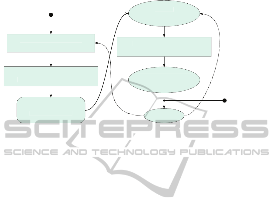
Figure 1: Flowchart of the plane estimation. Estimation algorithms are boxed by a rectangle, estimated variables are shown in
ellipses. The tracking block is shown in a box with round corners. To estimate the orientation of the plane a RANSAC based
outlier rejection is affected, followed by a Least Squares optimization on the inlying points. The orientation is tracked by a
Kalman Filter. The tracked orientation is used to fit a plane to the point cloud with another outlier rejection to find the distance
of the plane to the origin. From there the scale can be calculated knowing the height over ground of the camera. The scale
has to be reverted to the outlier rejection in order to determine the inlier threshold. The decoupling of the plane orientation
estimation and the plane distance estimation is advantageous since sceneries with short occlusion of the ground plane can be
bridged by the tracking.
the scale. Since we want to focus on user oriented ap-
plications we use a low-cost single-row laser scanner.
In order to calculate the scale we need to cor-
relate a metric measurement with an unscaled point
from the reconstruction of the scene. A basic idea
is the selective reconstruction of the point that cor-
responds to the hit point of the laser p in the image
I. This point is known by the laser to camera cal-
ibration, see section 5.3. Knowing the fundamental
matrix F of two consecutive frames I
0
and I by the
eight-point-algorithm we can calculate the epipolar
line l
0
in the first image I
0
corresponding to p with
l
0
= F p. The corresponding point p
0
in I
0
can then
be found economically by sampling key points along
this epipolar line and matching descriptors extracted
of their surroundings and the surrounding of p. As
descriptor a simple block matching or the descrip-
tor BRIEF (Calonder et al., 2010) are considered and
have yet to be evaluated. Knowing p and p
0
as well as
F and therefore the rotation and translation between I
and I
0
, we can reconstruct the 3d point corresponding
to p and extract the scale due to the metric measure-
ment of the laser scanner.
5.3 Laser to Camera Calibration
In order to know the image position of the points
where the laser beams hit an object, difference in pose
∆P between the camera and the laser scanner have to
be known. In our case, we use a low-cost laser scan-
ner. Its standard deviation of the range measurements
is very high, approximately 0.1m. Consequently tar-
get based calibration methods have a low chance of
success, which is why we rely on a proper vision
based method.
Our cameras do not have infrared filters so that
the laser-object intersection points can be recognized
in the image, see figure 2. To calibrate our device
we fix the position of the camera-laser unit and put a
planar object in front of it. Over time we move that
object slowly varying the distance of the object and
the sensor device between 0.2m to 4.0m. Our goal
is to extract the measured laser point from the image
and minimize the reprojection error between the re-
projected 3d laser points measured by the scanner and
the observed points in the camera image as shown in
equation 1.
argmin
P=(α,β,γ,t
x
,t
y
,t
z
)
∑
i
u − u
pro j
(P)
v − v
pro j
(P)
2
2
(1)
α,β,γ indicate the rotation angles and t
x
,t
y
,t
z
the trans-
lation vector. u
pro j
,v
pro j
denote the back projected 3d
laser scanner points and u,v are corresponding points
in the image.
A challenge poses the measurement point extrac-
tion. Especially at high distances the measured points
in the image can have a very low brightness whereas
VISIGRAPP2015-DoctoralConsortium
40
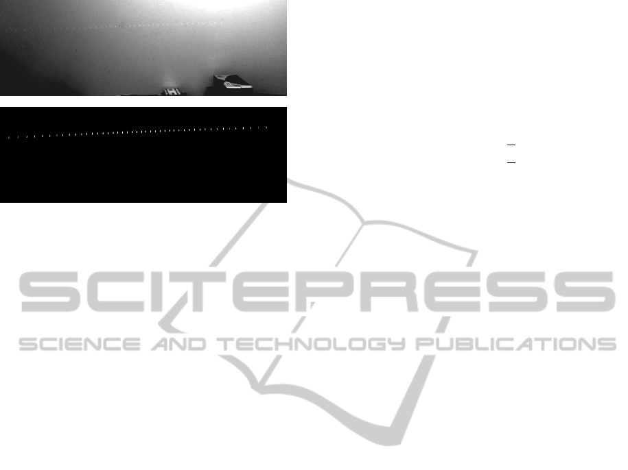
Figure 2: Points of the laser scanner seen in the camera
image in a darkroom. On top we see the scene with lights
on, in the lower image the light is turned off.
Figure 3: Overlapped images of laser scan measurements at
different distances. In red we see the manually marked lines
used for measurement extraction.
at small distances the points meld. To overcome this
we overlap the camera images from different points in
time, which results in a fan-like image. This fan rep-
resents the epipolar lines of the laser scanner in the
image. Next we can manually mark these lines and
extract pixels with maximum brightness in their prox-
imity. The overlapped image is shown in figure 3.
After convergence of the nonlinear minimization
problem posed in equation 1 we obtain the pose of
the laser scanner relative to the camera. A qualitative
evaluation of the calibration is given in figure 4.
5.4 Cyclist Motion Estimation
As described in section 4.2 we need to estimate the
trajectory of a cyclist detected in the image in order
to predict the collision between the automobile and
the cyclist. The cyclist’s position in image coordi-
nates can be estimated by novel algorithms developed
by Tian and Lauer (Tian and Lauer, 2014). Our goal
is to estimate the cyclist’s position in 3d coordinates.
In a first approach we model the cyclist by its po-
sition in 3d space, x, y, z and by its velocity v
x
,v
y
,v
z
.
We assume that its acceleration is small and model it
by the uncertainties of the velocity. Furthermore, the
cyclist moves on a plane that is parallel to the plane
spanned by z and x. Therefore we choose v
y
to be zero
and y constant with very small uncertainty. Thus our
problem is nearly two dimensional and more robust
than in three dimensional space, but with the advan-
tage that small changes in the ground plane inclina-
tion can still be modeled.
Using a pinhole camera model the image posi-
tion of a 3d point of the camera coordinate system
(x
l
, y
l
, z
l
)
T
is given by
u
v
= Intrin ·
x
l
z
l
y
l
z
l
1
(2)
Intrin is the intrinsic matrix of the pinhole cam-
era. Therefore an image point p given by u and v
maps onto a ray in 3d space.
By measuring the distance of the cyclist with a
range based method we can thus estimate the distance
from the cyclist to the camera and determine its po-
sition. Knowing the global camera pose due to the
ego-motion estimation, it is possible to express the
cyclist’s position (x, y, z)
T
in global coordinates.
x
l
y
l
z
l
= T (x) =
R(α, β, γ)
t
x
t
y
t
z
·
x
y
z
1
(3)
Hereby R denotes the rotation matrix and
(t
x
, t
y
, t
z
)
T
the translation vector of the camera rela-
tive to the origin.
However, the raw position estimate of the detected
cyclist does not attain our need of precision. Con-
sequently a method is needed for estimating the po-
sition of the cyclist more accurately. Moreover, the
LIDAR measurements are not synchronized with the
image capture. As a result the algorithm needs flex-
ibility regarding the incorporation of the range mea-
surement. Here we propose two suitable methods, the
first one being able to yield good results if the fre-
quency of the range measurements is high, the second
one being more suitable for low range measurement
frequencies.
5.4.1 Cyclist Tracking by an Unscented Kalman
Filter
The first method is tracking by an Unscented Kalman
Filter (UKF), a well established method for non-
linear tracking introduced by Wan (Wan and Van
Der Merwe, 2000). The state transition function
x
i+1
= f (x
i
) between two states x
i
and x
i+1
is here
defined as
x
i+1
= f (x
i
) =
x + ∆t · v
x
y + ∆t · v
y
z + ∆t · v
z
v
x
v
y
v
z
(4)
MonoscopicAutomotiveEgo-motionEstimationandCyclistTracking
41
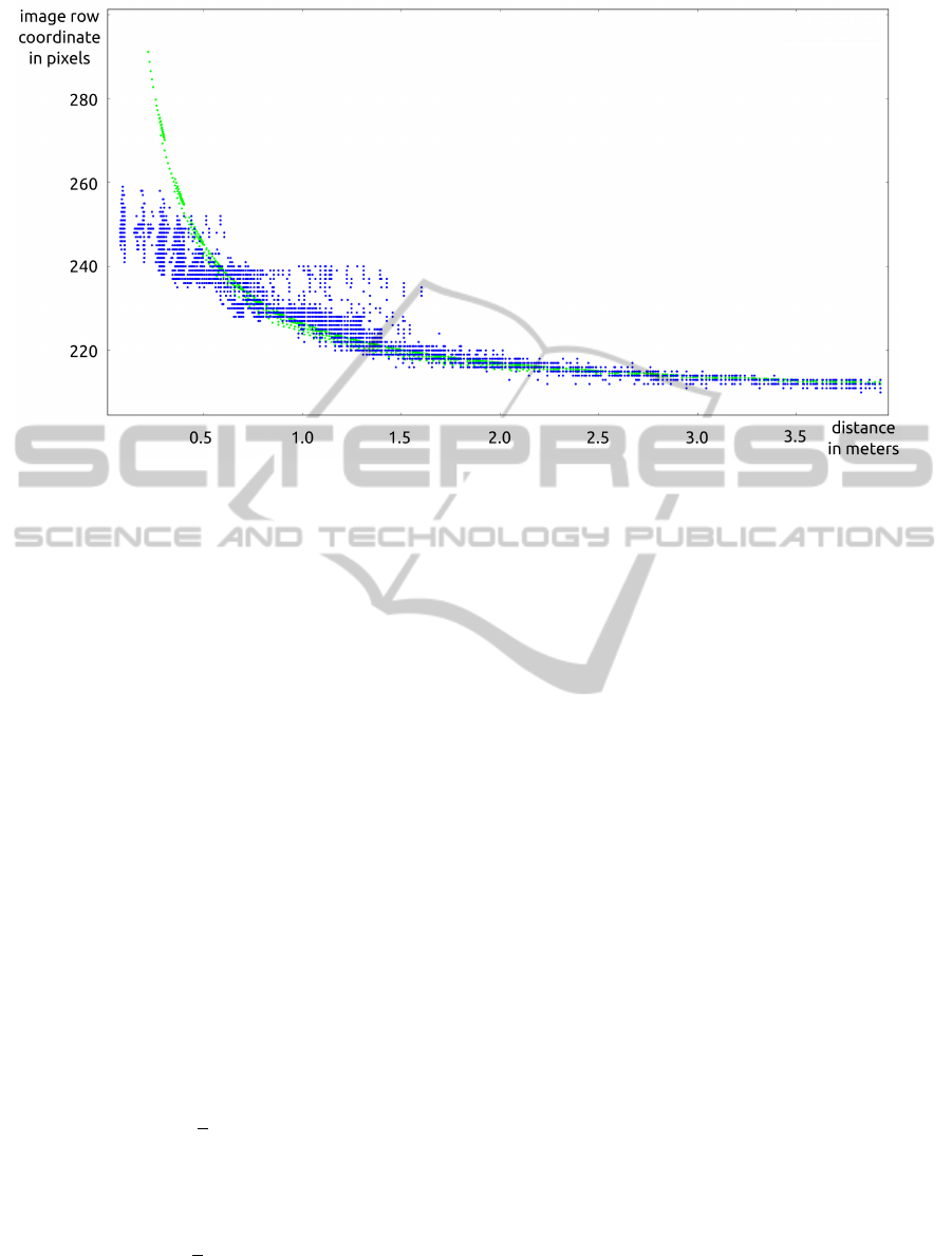
Figure 4: Evaluation of the laser scanner to camera calibration. Measured points in the image are shown in blue, 3d laser
scanner points that are reprojected using the calibrated pose are shown in green. We see that at distances up to 1.0m the
measurement points are very fuzzy. This is to one part caused by the noisy depth measurement of the laser scanner and to
another part caused by a time jitter due to the asynchronism of the laser scanning and the image capturing. However, at
distances from 1.5m on, the green curve and the blue curve fit well and therefore the calibrated pose between the laser scanner
and the camera is sufficiently accurate.
The state transition is linear in x but depends on the
time increment ∆t which changes from estimation to
estimation. The measurement function p
i,Meas
= h(x
i
)
for the position of the cyclist in the image is a nonlin-
ear function. In addition to that we denote the mea-
surement function for the depth d
i,Meas
= g(x
i
). First
the global position estimate x
i
, y
i
, z
i
at time i is trans-
formed to local camera coordinates by equation 3.
Since the local coordinates are chosen such as the z-
axis corresponds directly to the depth of the image we
therefore formulate
d
i,Meas
= g(x
i
) =
0 0 1
· T (x
i
) (5)
Then, we project the local position estimate
x
i,l
, y
i,l
, z
i,l
to the image by the pinhole model with
equation 2.
A critical point using Kalman Filters is the deter-
mination of the process noise covariance and the mea-
surement error covariance. We assume the standard
deviation of the acceleration of the cyclist in the direc-
tions x and y: σ
acc
= 1.0
m
s
. Thus follow the standard
deviations for the velocities and positions
σ
v
= ∆tσ
acc
(6)
σ =
1
2
∆t
2
σ
acc
(7)
Note that the process noise covariance is dependent
on the time difference between two measurements.
The process noise covariance Q is hence defined as
σ
2
0 0 σσ
v
0 0
0 0.01σ
2
0 0 0.01σσ
v
0
0 0 σ
2
0 0 σσ
v
σσ
v
0 0 σ
2
v
0 0
0 0.01σσ
v
0 0 0.01σ
2
v
0
0 0 σσ
v
0 0 σ
2
v
(8)
The scalar factors in front of the entries of the position
and the velocity in y-direction model the quasi planar
motion of the cyclist. In order to make the tracking
more robust the height of the cyclist can additionally
be detected and included in the tracking as a 7th es-
timation parameter. This gives us an idea of the dis-
tance of the cyclist to the camera but can only be used
to stabilize the depth tracking since the accurate met-
ric measures of cyclists vary. The measurement noise
covariance for both h(x) and g(x) is assumed to be
uncorrelated.
5.4.2 Cyclist Tracking by a Least Squares
Approximation
In this second method we approximate the cyclist’s
state by a sliding window of n camera frames at
points in time t
i
. In this window we assume con-
stant velocity of the cyclist. Therefore the assump-
tions here are stronger compared to the UKF in sec-
tion 5.4.1 where we allow a small variation in each
VISIGRAPP2015-DoctoralConsortium
42

frame. To calculate the position x = (x, y, z)
T
and ve-
locity v = (v
x
, v
y
, v
z
)
T
, we minimize the quadratic er-
ror
argmin
x,v
n
∑
i=1
k(x +t
i
v − p
i
)k
2
2
(9)
p
i
is the measured cyclist position in 3d world coordi-
nates at t
i
. Zeroing the first derivative respect to x and
v gives the classic Linear Least Squares equation
I · n I
∑
i
t
i
I
∑
i
t
i
I
∑
i
t
2
i
·
x
v
=
∑
i
p
i
∑
i
t
i
p
i
, i = 1 . . . n (10)
I denotes the identity of R
3
. The cyclist position p
i
is measured from the vehicle at position P
i
by a range
r
i
from the laser scanner and a direction w
i
from the
camera, from which follows
p
i
= P
i
+ r
i
w
i
, kw
i
k
2
= 1 (11)
Hereby we face the problem that we can not ob-
serve a range detection for each t
i
. Thus we have to
include an estimation for range detections. This is
done by projecting the estimated local cyclist position
x +t
i
v − P
i
at each time instant t
i
on the direction w
i
.
With w
T
i
x
i
w
i
= w
i
w
T
i
x
i
= WW x
i
we conclude the es-
timation for the cyclist position and velocity as shown
in algorithm 1.
The strong assumption that the velocity is constant
in a sequence of frames, renders this method less flex-
ible compared to the UKF, for which small variations
are allowed for each frame. Therefore the UKF is
more appropriate if a lot of range measurements are
available. However, if only few range measurements
are made, i.e. at a frequency of 1 Hz and less, this
method is more robust. A qualitative comparison of
both algorithms is given in figure 5. A quantitative
evaluation is work in progress.
6 EXPECTED OUTCOME
The declared goal of this PhD thesis is to lever-
age monoscopic Visual Odometry to broad appliance.
From our point of view the key to that is the solution
of the scale ambiguity. Therefore the expected result
of this PhD project is a monoscopic Visual Odometry
framework with very small drift due to simple addi-
tional sensors and the correct estimation of the metric
scale. This will allow to instantiate full-fledged Vi-
sual Odometry algorithms using a monocular camera
system, which is a favorable platform on account of
its ease of use and low price as well as its broad appli-
cability. Utilizing this potential, a variety of applica-
tions can be put into practice, which could comprise:
Algorithm 1: Algorithm for estimating the cyclist po-
sition by a Linear Least Squares method with latent
variables.
Ensure: t {Vector of time increments, size n}
Ensure: w {Vector of directions camera to cyclist,
size n}
Ensure: P {Vector of camera position in global co-
ordinates, size n}
Ensure: r {Vector of distances of camera to cyclist,
less than n valid values}
M ← zero matrix of R
6x6
C ←
0 0 0 0 0 0
T
I ← identity of R
3x3
for i ← 1 . . . n do
M ← M +
I t(i)I
t(i)I t(i)
2
I
C ← C +
P(i)
t(i)P(i)
if Observed then
C ← C +
r(i)w(i)
t(i)r(i)w(i)
else
WW ← w(i) · w(i)
T
M ← M −
WW t(i)WW
t(i)WW t(i)
T
·W
C ← C −
WW · P(i)
t(i) ·WWP(i)
end if
end for
XV ← M
−1
C {6d target state}
• The trajectory estimation of an endoscopic system
from which objects in the scenery, such as medi-
cal anomalies, can be observed and reconstructed.
Since inside the human body the camera would
be placed in a dense environment a single-laser-
beam range finder could suffice for determining
the scale.
• Establishing a high precision and low-cost naviga-
tion system by fusing monoscopic Visual Odom-
etry with GNSS data, which would be applicable
in autonomous driving, general robotics and en-
hanced reality.
A very important application, a lifesaving cyclist
detection and tracking system, is already on the edge
of realization. We will establish and test this system
within the next year as a part of the ABALID project
of the Federal Ministry of Education and Research of
Germany (ABALID, 2014).
MonoscopicAutomotiveEgo-motionEstimationandCyclistTracking
43
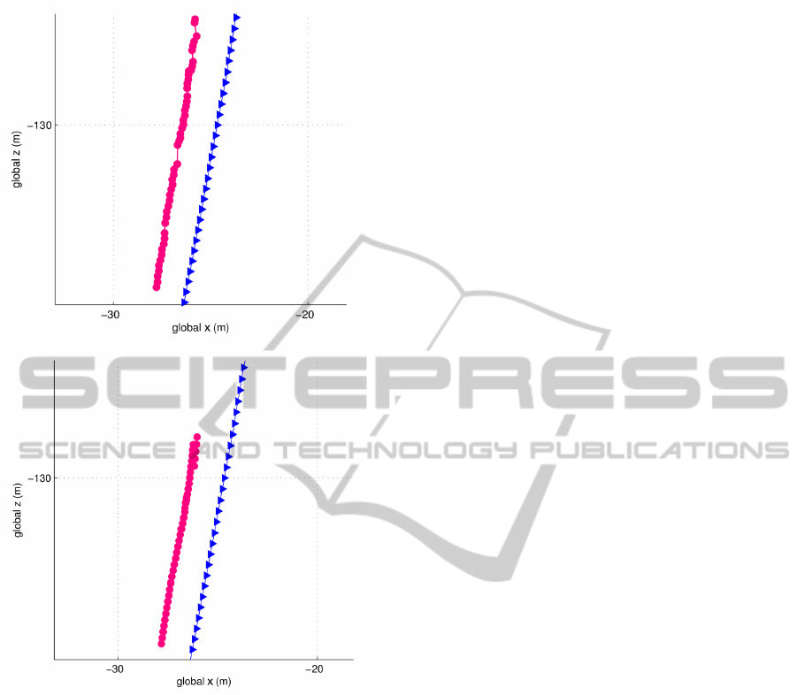
Figure 5: Comparison of the cyclist tracking with the Un-
scented Kalman Filter on top and the Linear Least Squares
method with latent variables at the bottom at a range mea-
surement frequency of 1 Hz and a camera measurement fre-
quency of 10 Hz. The Linear Least Squares method tends
to smoother results. However, at z = −130 the Linear Least
Squares method fails because of an inaccurate camera mea-
surement, the UKF however can continue. For high range
measurement frequencies the tracking with the UKF seems
more appropriate, for lower frequencies the Linear Least
Squares is the method of choice.
REFERENCES
ABALID (2014). Homepage of the abalid project.
http://abalid.de/. Accessed: 2014-12-10.
Calonder, M., Lepetit, V., Strecha, C., and Fua, P. (2010).
Brief: Binary robust independent elementary fea-
tures. In Computer Vision–ECCV 2010, pages 778–
792. Springer.
Engel, J., Sch
¨
ops, T., and Cremers, D. (2014). Lsd-slam:
Large-scale direct monocular slam. In Computer
Vision–ECCV 2014, pages 834–849. Springer.
Forster, C., Pizzoli, M., and Scaramuzza, D. (2014). Svo:
Fast semi-direct monocular visual odometry. In Proc.
IEEE Intl. Conf. on Robotics and Automation.
Fraundorfer, F. and Scaramuzza, D. (2012). Visual odom-
etry: Part ii: Matching, robustness, optimization,
and applications. Robotics & Automation Magazine,
IEEE, 19(2):78–90.
Geiger, A., Ziegler, J., and Stiller, C. (2011). Stereoscan:
Dense 3d reconstruction in real-time. In IEEE Intelli-
gent Vehicles Symposium, Baden-Baden, Germany.
Hartley, R. and Zisserman, A. (2010). Multiple View Geom-
etry. Cambridge University Press, 7th edition.
Hartley, R. I. (1997). In defense of the eight-point algo-
rithm. Pattern Analysis and Machine Intelligence,
IEEE Transactions on, 19(6):580–593.
Klein, G. and Murray, D. (2007). Parallel tracking and map-
ping for small ar workspaces. In Mixed and Aug-
mented Reality, 2007. ISMAR 2007. 6th IEEE and
ACM International Symposium on, pages 225–234.
IEEE.
Scaramuzza, D. and Fraundorfer, F. (2011). Visual odom-
etry [tutorial]. Robotics & Automation Magazine,
IEEE, 18(4):80–92.
Tian, W. and Lauer, M. (2014). Fast and robust cyclist de-
tection for monocular camera systems.
Wan, E. A. and Van Der Merwe, R. (2000). The unscented
kalman filter for nonlinear estimation. In Adaptive
Systems for Signal Processing, Communications, and
Control Symposium 2000. AS-SPCC. The IEEE 2000,
pages 153–158. IEEE.
VISIGRAPP2015-DoctoralConsortium
44
