
Distributed Techniques for Energy Conservation in Wireless Sensor
Networks
∗
Mohamed Abdelaal
†
System Software and Distributed Systems Group, Carl von Ossietzky University of Oldenburg, Oldenburg, Germany
1 STAGE OF THE RESEARCH
The PhD program has commenced on December
2012 for three years where the graduation is expected
to be in 2016. The main theme of this work is
to improve the energy efficiency of Wireless Sen-
sor Networks (WSNs). The thesis has multiple ap-
proaches tackling the main sources of energy con-
sumption in WSNs. These approaches are classi-
fied into three main roots: ”‘Energy-cheap”’ data
aggregation, Hardware optimization and Predictive
self-adaptation WSNs. Currently, we have already
achieved a reasonable progress as can be seen below.
2 OUTLINE OF OBJECTIVES
Generally, the integration of sensor nodes (SNs), gate-
ways and software forms a sensor network. The spa-
tially distributed SNs may have numerous on-board
sensors whose outputs are wirelessly conveyed via
multi-hop link to a gateway. The software manages
the allocation of node resources in a controlled man-
ner. The ideal characteristics of a typical WSN are
low power consumption, scalability, dependability,
remote configuration of SNs, programmability, fast
data acquisition, security, and fidelity of data flow
over the long term and with little or no maintenance
(Akyildiz et al., 2002).
The crux behind this work is to extend the lifetime
expectancy of wireless sensor networks (WSNs). In
particular, we target exploiting the trade-off between
reducing certain quality-of-service (QoS) measures to
a degree still tolerable by the application (such as, for
example, precision and latency) and maximizing the
∗
This research is funded by the German Research Foun-
dation (DFG GRK 1765) through Research Training Group:
System Correctness under Adverse Conditions (SCARE),
http://www.scare.uni-oldenburg.de/
†
Supervisor: Prof. Dr.-Ing. Oliver Theel, Department of
Computer Science, System software and Distributed Sys-
tems Group, Carl von Ossietzky University of Oldenburg,
Germany, theel@informatik.uni-oldenburg.de
application’s lifetime. For satisfying these objectives,
the following sequential steps are addressed. At the
outset, an elaborated survey is sketched to aggregate
the diverse endeavors in this context. This survey
paves the way for identifying the weak points to be
tackled. The PhD thesis is structured from three main
categories:
• Cat I: “Energy-cheap” Data Aggregation. In
this category, we have proposed a new data com-
pression technique based on the so-called fuzzy
transform. Moreover, we have improved its accu-
racy to be comparable with the well-known data
reduction techniques. In the sequel, we are inter-
ested in bridging the fidelity gab between lossy
and lossless compression techniques. Thus, we
can improve the feasibility of adopting high com-
pression ratios with high degree of correctness.
Distributed data aggregationis also tackled via ex-
ploiting the spatio/temporal correlation among the
deployed sensors. The dynamic time warping al-
gorithm has been modified to suppress the redun-
dant messages.
• Cat II: Hardware Optimization. In this cate-
gory, we have commenced by the sensing module
where reliable virtual sensing has been proposed
to reduce the overheadof “energy-expensive”sen-
sors. Afterward, the energy consumed by the re-
ceiver during idle listening will be tackled. We
are interested in designing a subconscious mode
in which the receiver frequency is reduced. How-
ever, a challenge of detecting the incoming pack-
ets, without violating the Nyquist-Shannon sam-
pling theorem, will emerge.
• Cat III: Predictive Self-adaptation WSNs. In
this category, we implement a proactive sensor
network which overcomes the flaws of reactive
networks. Reactivity adds a long accumulated de-
lay between detecting an event and responding to
it. Hence, we combine the predictive reasoning
and self-adaptation to improve the procedure by
which sensor nodes deal with the network dynam-
ics.
The remainder of the paper is organized as fol-
9
Abdelaal M..
Distributed Techniques for Energy Conservation in Wireless Sensor Networks.
Copyright
c
2015 SCITEPRESS (Science and Technology Publications, Lda.)

lows. Section 3 elaborates on the problem of energy
efficiency and our definitions in this context. Sec-
tion 4 briefly presents the previousendeavors for tack-
ling the WSNs energy problem. Section 5 presents
our methodologies (summarized in Tabel 1) for mit-
igating the headache of energy efficiency in WSNs.
Finally, section 6 discusses the expected outputs of
the PhD thesis.
Table 1: Indexing the proposed energy efficiency methods.
Section Title Category
5.1 Fuzzy Data Compression I
5.2 Reliable Virtual Sensing II
5.3 IEEE 802.15.4 Refinement II
5.4 DTW-based Data Aggregation I
5.5 Predictive Self-adaptation WSNs III
3 RESEARCH PROBLEM
Energy efficiency is a fertile research area. The
WSN literature has been submerged with many en-
ergy conservation and harvesting techniques. Nev-
ertheless, most of these approaches are application-
dependent, preventing any sort of standardization.
Moreover, some energy dissipation sources, such
as transceiver’s operating frequency, have not been
strongly addressed. Adopting novel ideas, as those
presented in this work, could highly improve the
WSN’s lifetime.
Symbolically, the energy consumption problem
can be denoted as shown in Eq. 1. Under the assump-
tion Asm of allocating an amount of energy for each
SN, a system Sys (operating in the environment Env)
has to satisfy the user’s specifications Spec. These
demands could be defined as an integer linear pro-
gramming problem as given in Eqs. 2-4. Specifically,
Eq. 2 minimizes the total energy consumption of a
WSN consisting of k nodes with two criteria:
Asm ⊢ (Env k Sys) sat Spec (1)
minimize(
k
∑
SN=1
(P
useful
(SN)) + P
wasted
(SN)) (2)
provided that
η(SN) ≥ δ ∀s ∈ WSN (3)
100% ≥ β ≥ 100− ψ% ∀s ∈ WSN (4)
• The lifetime (η) of each SN has to conform with
the minimum time δ required to complete the as-
signed task as expressed in Eq. 3.
• The WSN performance β (defined in terms of the
QoS parameters) should satisfy the minimum ap-
plication requirements. Hence, a small space ψ
could tolerate the trade-offs as defined in Eq. 4.
Figure 1 depicts a comprehensivetaxonomy of the
various energy consumption sources in WSNs. The
green boxes reveals the targeted sources to be tackled
in this work. Specifically, energy conservation is ac-
complished via deliberately trading-off the WSN life-
time versus other QoS parameters such as precision
and latency.
4 STATE OF THE ART
A rationale methodology commences with scanning
the literature to identify the gabs. Accordingly, a new
taxonomy has been established including the recent
endeavors (Abdelaal and Theel, 2014). Initially, en-
ergy management in WSNs has been divided into en-
ergy harvesting and energy conservation. The former
denotes scavenging the surrounding energy sources
to fully (or partially) energize the sensor nodes. In
most cases, the harvested power is relatively defi-
cient. Furthermore, external power supply sources, in
many cases, exhibit a non-continuous behavior which
can cause system malfunctioning. However, ”‘green
WSNs”’ are feasible through improving the harvest-
ing mechanisms and minimizing the consumption.
As can be seen in Fig. 2, the energy saving ap-
proaches can be classified according to its scope into:
Local, and Global techniques. The former elaborates
the methods for mitigating the energy consumption
due to local energy-waste sources such as data redun-
dancy, non-optimal HW/SW congurations, etc. The
latter comprises a collection of distributed energy sav-
ing techniques which involveoptimization of commu-
nication and networking protocols.
Due to the lake of space, we could not elaborate on
these energy efficiency techniques. However, inter-
ested readers could find more details in (Abdelaal and
Theel, 2014). Next, we present our proposed ideas for
locally reducing the energy consumption of the sensor
nodes.
5 METHODOLOGY
Based on this classification, many ideas have emerged
to optimize the nodes’ operation. Actually, local data
compression significantly affects the energy profile,
however, the previous techniques are either ill-suited
for hardware implementations or overly dedicated.
Therefore, the thesis embarks on a novel compres-
sion concept which exploits the advantages of existent
techniques and avoids their shortcomings.
SENSORNETS2015-DoctoralConsortium
10
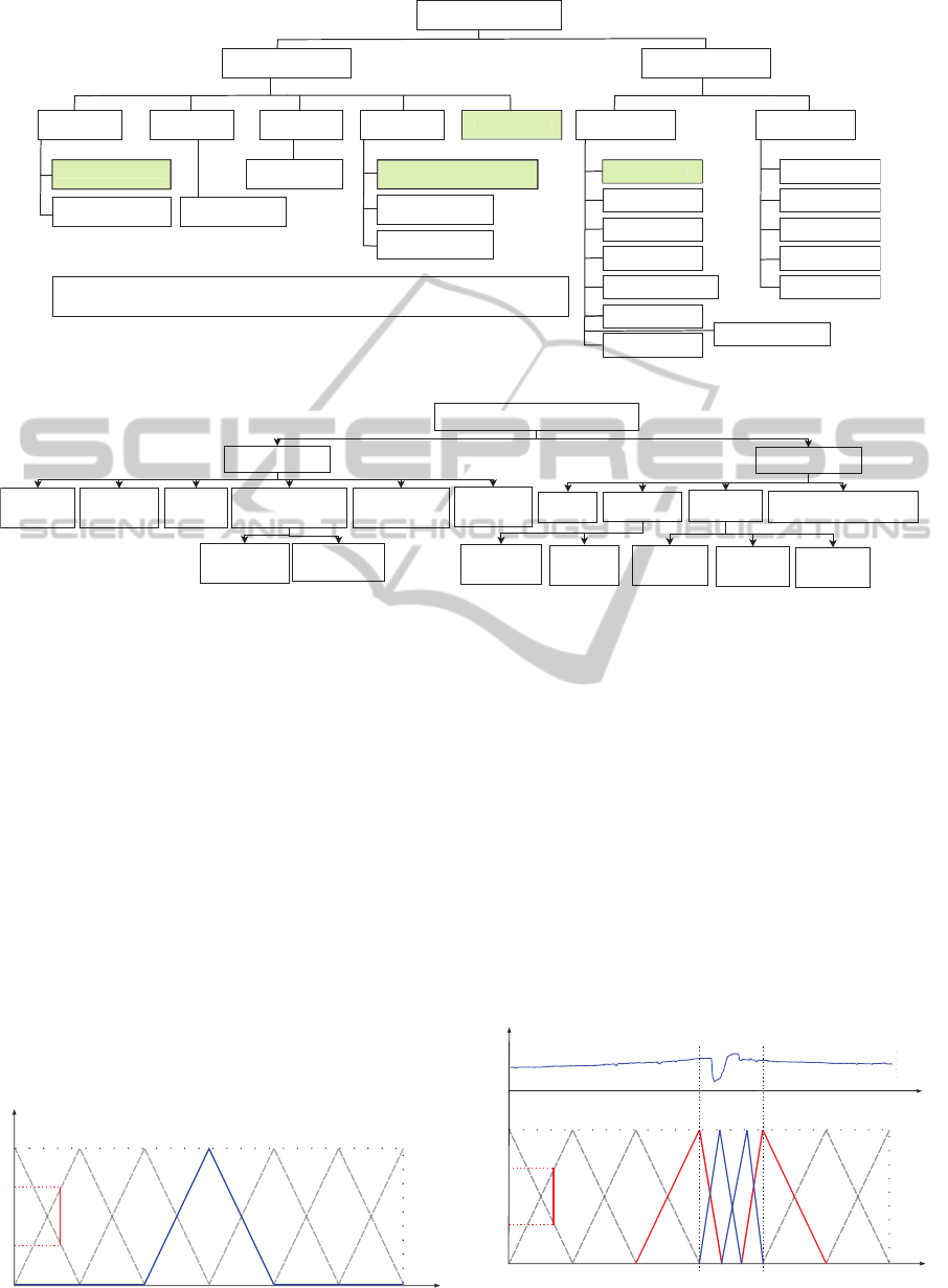
Energy Consumption
Component Level
Functional Level
Sensors MCU Memory Radio
State Switching Local Global
Idle Listening
Protocol Overhead
Overhearing
Collision
Nieghbor Monitoring
Security
Routing
Protocol Overhead
Topology Control
Packet Loss
Read/Write (N
op
)
Overemiting
Phenomena Detection
Redundancy
Sampling (f
s
), ADC
Transmit/Receive (b, d, r, t)
Modulation Scheme
Startup Energy
Computation (N
op
)
where f
s
= sampling frequency, N
op
= number of clock operations, b = number of bits to
be trannsmitted, d = distance between sensder & receiver, r = data rate, t = Transmit power
Phenomena Detection
Transmit/Receive (b, d, r, t)
State Switching
Idle Listening
Software Inefficiency
Figure 1: Taxonomy of energy consumption sources in WSNs.
Energy-preservation Techniques
Global
Local
Mobility
Distributed
Compression
Data
Prediction
Redundancy
Control
Duty Cycling
MAC
Optimization
Energy-efficient Networking
HW/SW
Optimization
Data
Reduction
Virtual
Sensors
Energy-efficient
Cognitive Subsystem
Memory Leakage
Control
Scaling
Cognitive
Radio
Data Acquisition
Data-driven
Aggregation
Protocols
Figure 2: Taxonomy of energy conservation techniques in WSNs.
5.1 Fuzzy Compression
In this section, we start the first category of the PhD
hierarchy. A local data compression technique based
on the so-called Fuzzy transform (F-transform) has
been proposed. The F-transform usually converts a
continuous (or discrete) signal into an n-dimensional
vector (Perfilieva, 2004). In (Abdelaal and Theel,
2013a), the fuzzy compression technique (FTC) was
adapted in line with the measured phenomena. Learn-
ing the data significance via thresholds was a straight-
forward technique which can be upgraded in possible
extensions. Figure.3 depicts a uniform basic function
composed of a set of triangular membership compo-
nents. The shape of such basic function determines
the approximating function. Thus, FTC is a suitable
compressor for linear and nonlinear sensor data.
The results showed an adequate lifetime gain,
x
1
x
k
0
1
x
0
= a x
n
= b
p
1-p
A
1
A
2
A
k
A
n
Figure 3: Structure of the basic function.
however, the FTC should be compared to ensure its
outweigh. Therefore, the FTC is then contrasted
to the lightweight temporal compression technique
(LTC) in (Bashlovkina et al., 2015). In this paper,
a new algorithm, referred to as FuzzyCAT, has been
applied to minimize the recovery error even with high
compression ratios via hybridizing the approximating
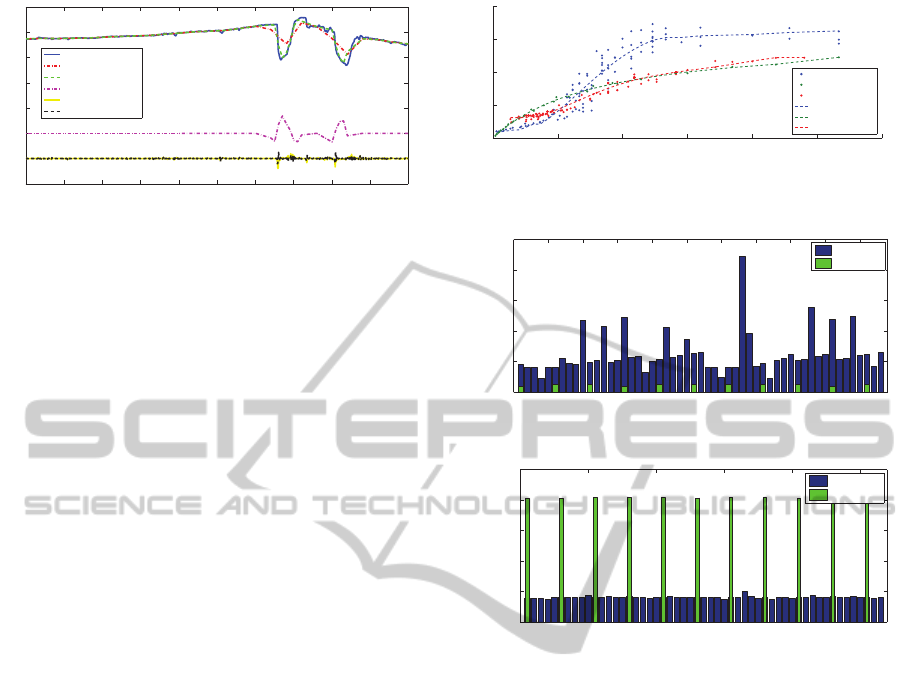
function. Figure 4 demonstrate the fluctuations track-
ing in light of the readings second derivative. The
sample signal is shown on top, and the fuzzy sets con-
structed by FuzzyCAT for that signal are displayed
on the bottom. On the half periods where the signal
is smooth, the regular membership functions are ap-
plied. In the half period where fluctuations were de-
tected, narrower basic functions are applied (in blue).
x
1
x
k
0
1
x
0
= a x
n
= b
p
1-p
A
1
A
2
A
k
A
n
40
45
50
55
t
Light Intensity
Figure 4: Adapting the basic function via tracking the fluc-
tuations.
DistributedTechniquesforEnergyConservationinWirelessSensorNetworks
11
0 100 200 300 400 500 600 700 800 900 1000
10
0
10
20
30
40
50
60
Timestamp
Absolute Value
Actual Data
FT
FuzzyCAT
Diff (FT, FuzzyCAT)
First Derivative
Second Derivative
Figure 5: Comparison between FTC, and FuzzyCAT.
Figure 5 compares the performance of the regular
FTC and the FuzzyCAT algorithm on a segment of the
temperature signal from the Berkely lab dataset (lab,
2014). Both algorithms were set to compress the 1000
data points into 26 coefficients, while FuzzyCAT adds
three additional basic functions per half period when
needed. The scaled pink line, representing the dif-
ference between the signal reconstructed by the reg-
ular FTC and FuzzyCAT, reveals that the algorithms
yielded identical results on most of the segment, only
deviating on the intervals with high fluctuations. The
FTC yields compression ratio of 38.46, with normal-
ized RMSE of 8.72%. The adaptive transform added
9 extra membership functions, decreasing the com-
pression ratio to 28.57 and bringing the normalized
RMSE down to 4.22%. Adding extra membership
functions cut the RMSE by more than half - a 52% de-
crease, while the resulting compression ratio was only
25% percent smaller than the original. Thus, Fuzzy-
CAT exhibits a compelling advantage over the regular
F-transform.
Figure 6 shows a fidelity comparison between
FTC, LTC, and FuzzyCAT methods. Note that de-
pending on the error margin, LTC can yield different
reconstruction errors with the same compression ra-
tio. LTC performs best, when CR is under 50, after
which the FuzzyCAT is likely to perform just as well.
For a CR above 75, FuzzyCAT and FTC outperform
the LTC technique.
Figures 7-8 depict the results of a set of experi-
ments on TelosB nodes. has confirmed the superiority
of FuzzyCAT over the LTC technique where transmis-
sion cost of the FuzzyCAT is 96% less than that of the
LTC at the expense of 10.28% processing increase.
Analyzing the FuzzyCAT superiority reveals that
the algorithm requires conveying a single array of
compressed measurements per data acquisition win-
dow, whereas the LTC transmits a separate packet for
each approximated linear segment. Thus, FuzzyCAT
efficiently spreads the overhead involved in sending
each packet. This property of FuzzyCAT also re-
sults in periodicity of transmissions, unlike the un-
predictable nature of LTC’s sending patterns. Peri-
0 50 100 150 200 250 300
0
5
10
15
20
Compression Ratio
Normalized RMSE (%)
LTC
FTC
FuzzyCAT
Poly(LTC,5)
Poly(FTC,5)
Poly(FuzzyCAT,5)
Figure 6: Normalized error versus compression ratio of
LTC, FTC, and FuzzyCAT.
0 5 10 15 20 25 30 35 40 45 50
0
0.01
0.02
0.03
0.04
0.05
Packet Epoch
Power Consumption (mW)
LTC
FuzzyCAT
Figure 7: Transmission power consumption.
0 10 20 30 40 50
0
0.005
0.01
0.015
0.02
0.025
Packet Epoch
Power Consumption (mW)
LTC
FuzzyCAT
Figure 8: Processing unit power consumption.
odicity of transmissions is valuable because it allows
(1) to implement scheduling algorithms thus minimiz-
ing idle listening and packet collisions and (2) to eas-
ily detect lost packets: the sink expects a packet and
sends a NACK message if the packet did not arrive in
time. Neither feature can be used with LTC since the
packets are sent irregularly (Raza et al., 2012).
As possible extension in this arena demands
widening the picture to figure out the pros and flaws
of lossy and lossless techniques. Specifically, a WSN
is technically efficient whenever it functions up to
its expected lifetime (successful energy conservation)
along with achieving high degree of data fidelity.
Generally, the lossy compressors outperform the loss-
less counterpart in terms of the compression ratios.
Nevertheless, their accuracy is still a headache stands
against boosting the compression ratio. Hence, we
introduce a general module for pre-conditioning the
sensor data prior to compression. Thus, the ”‘down-
ward spiral”’ between compression ratios and recov-
ery accuracy could be broken. The crux is to quick-
sort the sensor data prior to being lossy-comprised.
This idea bases on the fact that lossy compressors
prominently resemble the behavior of low pass fil-
SENSORNETS2015-DoctoralConsortium
12

ters. The recovery mechanism comprises encoding
the data indices using a lossless approach. Two meth-
ods have been examined including reversible data hid-
ing and byte-pair encoding. Fig 9 depicts encoding
the data indices within a matrix through tracking the
horizontal and vertical steps. These steps are then
converted into binary representation by following Ta-
ble 2. For instance, the red steps in Fig 9 is encoded as
0001100100000110000000100000110010001. Data
hiding is used to indirectly shorten this bit stream into
only 32 bits. This method divides the stream into two
variables U and V. Afterward, it embeds v into U ex-
ploiting the frequent zeros (Kim, 2009).
Original Indices
Sorted Indices
a
1
a
2
a
3
a
4
a
5
a
6
a
1
a
2
a
4
a
6
a
7
a
8
a
8
a
7
a
5
a
3
Figure 9: Indirect encoding of the sensor data indices.
Table 2: Definitions of the various matrix transitions.
Symbol Transition
0 Vertical
1 Horizontal & directed downward
11
Horizontal & directed upward
A dictionary-based approach could save more bits
at the expense of skipping infrequent probabilities.
Table 3 depicts an example of dictionary composed
of the most frequent symbols. Other probabilities
such as 001, 100, and 101 is rounded to the closest
value in the dictionary. Following this method, the
bit stream is compressed from 37 bits to only 24 bits.
The proposed technique will be examined for low fre-
quency data (i.e. temperature and humidity readings)
and high frequency data (vibration data sets). More-
over, real experiments with the TelosB sensor nodes
could verify the accuracy improvement.
Several WSNs applications, on the other hand,
suffer from the high consumption of the sensing unit.
Accordingly, adaptive sampling techniques were in-
troduced to mitigate this burden at the expense of in-
creasing the event-miss probability. Hence, we devel-
oped a novel idea to prune the relationship between
Table 3: Dictionary-based compression.
symbol Probability (%) Code
000 50 00
010 16.7 01
011
16.7 10
110 8.3 11
energy consumption and event-miss probabilities.
5.2 Virtual Sensing
The work in this section belongs to the second cate-
gory of the PhD hierarchy. The amount of energycon-
sumed by sensor node’s components is application-
dependent. For instance, environmental monitoring
may utilize passive, energy-efficient sensors and may
require periodic transmission of the collected data.
In this setting, radio communication consumes the
majority of the residual energy (Oliveira and Ro-
drigues, 2011). In other settings, the sensor unit may
dominantly contribute to battery depletion, as it may
(1) utilize active sensors, such as µ-radars and laser
rangers, or “energy-hungry” passive sensors, such
as chemical and biological sensors (Li-zhong et al.,
2011), (2) demand high-rate and highly accurate A/D
converters, e.g. for acoustic or seismic transducers
(Akyildiz et al., 2005), or (3) prohibit energy-saving
sleep modes due to long data acquisition.
Virtual sensing is a novel technique for decreas-
ing the sensing unit energy consumption and simulta-
neously slashing the event-miss probability. Techni-
cally, virtual sensing digitally manipulates the outputs
of low-power hardware sensors to obliquely mon-
itor a phenomenon which could be directly mea-
sured via “energy-hungry” sensors. The energy gain
is cultivated from deactivating the main “energy-
hungry” sensor and instead monitoring the required
phenomenon via the virtual sensor. Triggering the
main sensor is done to guarantee a degree of relia-
bility.
In (Abdelaal et al., 2014), a technique, referred
to as EAVS, has been proposed and a case study of
gas leaks detection was given. The gas sensor could
be replaced by a set of light and temperature sensors
and a chemical film whose color is altered with the
existence of gases. Figure 10 shows a flowchart of
such virtual sensor. As can be seen, the sensing mod-
ule’s structure is changed in light of the virtual sen-
sor detection. Moreover, the virtual sensors dynam-
ically sleep to further conserve energy. Probabilistic
model checking was customized to estimate the gain
in terms of the saved energy and the detection latency.
Figure 11(a) compares the energy consumed by the
DistributedTechniquesforEnergyConservationinWirelessSensorNetworks
13
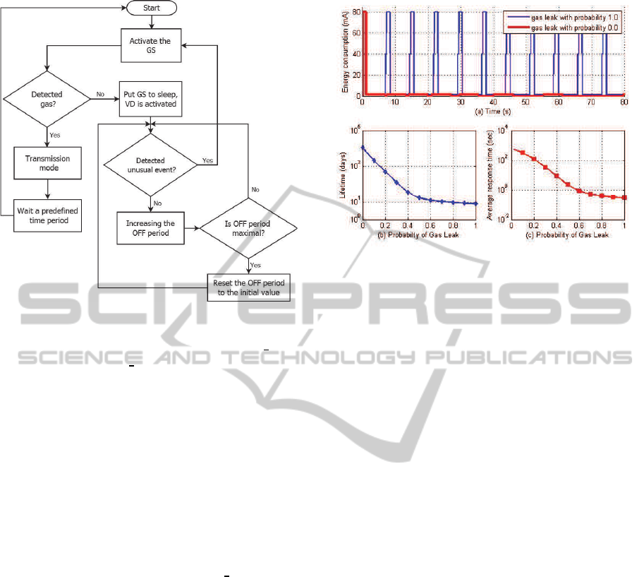
Figure 10: Virtual sensing flowchart.
sensing module gas leak probability of 0 (case
0: no
gas leaks) and 1 (case 1: always gas leaks). Logi-
cally, the latter is the worst case, however, the energy
consumption is highly reduced. Figure 11(b) demon-
strates the lifetime of a SN with different probabil-
ities. It gradually decreases with increasing the gas
leak probability. Our approach increase the lifetime
by 58 times more than that of the naive technique de-
scribed in (Somov et al., 2011). Nevertheless, EAVS
relatively suffers from the stretching in the response
time compared with a naive sub-system. The aver-
age response time is defined as the average period re-
quired for the sensor to react to a sudden change in
the quantity of interest. As can be seen in Fig. 11(c),
EAVS has a long response time in case
1 due to the
doubling the OFF periods. Notwithstanding, the re-
sponse time becomes shorter when the leaks are more
frequent. The worst case, in EAVS, is approximately
10 minutes compared with 2 minutes in (Somov et al.,
2011) (without leaks). However, the response time of
our approach can be shortened by reducing the OFF
periods.
Reliability of such systems composed of vir-
tual and real sensors should be guaranteed. At
a first glance, the replacement of real sensors
S by virtual sensors V = f(h
1
,..., h
n
) appears to be
reasonable and simple. However, utilizing n virtual
sensors could be a precision shortcoming where a
sensing quality set Q = {q
1
,..., q
n
} may have a nega-
tive impact on the detection probability of important
events. Especially when these replacements consist of
an orchestration of heterogeneous sensors like mag-
netic, radar,thermal, acoustic, electric, seismic, or op-
tical sensors. Thus, the quality of these sensors has to
Figure 11: Evaluating the virtual gas sensor.
be taken into account by the decision logic.
In (Abdelaal et al., 2015), a novel approach is
proposed to improve the virtual sensing reliability.
we focused on the quality of one particular set of
sensors and show how this set can replace an en-
ergy hungry sensor under certain quality aspects. An
ontology on sensor-environment relationships is uti-
lized to automatically generate rules before deploy-
ment to switch between real and virtual sensors. We
illustrate the general approach by a case study: we
show how reliable virtual sensing could reduce the
energy consumption and event-miss probabilities of
object tracking applications. Seismic sensors and a
dynamic time-warping algorithm shaped the virtual
object tracking sensor. Later, our approach will be
extended to show how the quality of a complex set of
heterogeneous sensors can be estimated using a sen-
sor relationship ontology.
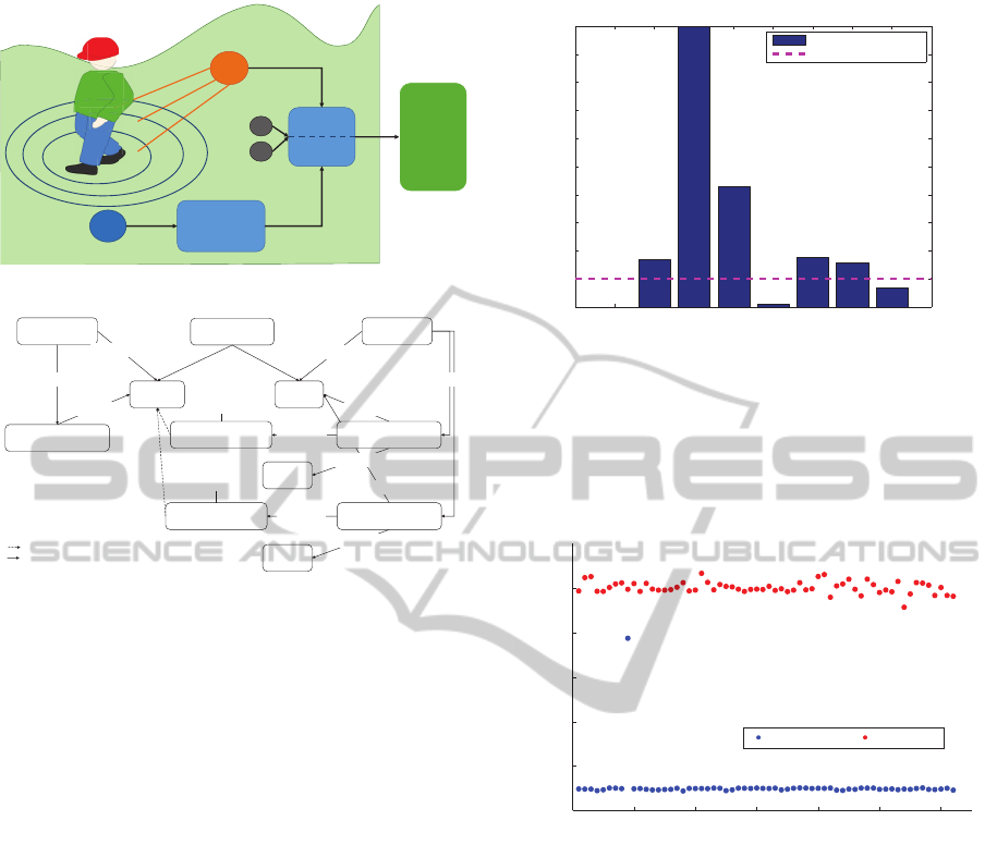
Figure 12 shows an object tracking system con-
sists of real and virtual sensors. The outcomes from
Omni-directional seismic sensors (sequence A) are
to trigger a well-known pattern matching algorithm,
called a dynamic time-warping. The key idea underly-
ing the virtual sensor V is to stretch (or compress) the
seismic trace until it best matches one of the reference
traces in the codebook (B
1
,.., B
z
). The quality estima-
tion mechanism utilizes secondary sensors to monitor
the quality of sensors. Based on this quality, the rules,
generated by the ontology, determines the well-suited
sensor. The switching decision between real sensor
S and virtual sensor V is affected by the sensing re-
liability and precision. In our concrete case, we can
model the relationships between the participating sen-
sor as shown in Fig. 13. The modeled relationships
are transformed into formulas to estimate the current
qualities.
DTW precision has been examined prior to be
SENSORNETS2015-DoctoralConsortium
14
Quality
estimation
Sensor
selection
Pattern
Matching
Radar
Sensor
Seismic Sensor
Application
Secondary
Sensors
object
detection
object
detection
Figure 12: System structure with real and virtual sensors.
Cluster
<Feature of Interest>
Temperature Sensor
<Sensing Device>
Seismic Sensor
<Sensing Device>
Temperature
<Property>
Vibrations
<Property>
value
<Measurement Capability>
pattern
<Measurement Capability>
Good
<Accuracy>
Not Working
<Temperature, Condition>
Bad
<Accuracy>
pattern
<Measurement Capability>
Working
<Temperature, Condition>
observes
Temperature >= 0
Temperature < 0
has Measurement Capability has Measurement Capability
observes
in Condition
in Condition
has Measurement Property
has Measurement Property
for Property
for Property
for Property
< > : Instance
: Inheritance
: Relationship
Figure 13: Ontology of the Virtual object tracker.
incorporated into the virtual sensor. At the outset,
an Arduino UNO board has been utilized to sample
seismic patterns from a LDT piezoelectric vibration
sensor. Different measuring scenarios of speed 0.5
m/sec have been considered. Figure 14 depicts sam-
ple of precision results obtained from contrasting the
codebook to some targeted and non-targeted patterns.
The vertical line denotes the normalized DTW dis-
tance between the measured pattern T1 and the code-
book patterns. Knowing that DTW(A,A) = 0, pat-
tern A
indoor
is matched with A
outdoor
to clarify the
process of selecting the best match. Obviously, the
DTW algorithm has successfully matched the indoor
and outdoor pairs via adopting the minimum DTW
inter-distance.
Figure 15 depicts the energy consumed via one
round for performing the liteDTW algorithm and
transmitting the minimum distances. Within 63
rounds, the processing consumes approximately 35%
more energy than transmission due to the time over-
head of the DTW algorithm. Hence, a possible
extension of this work may explore indexing as a
method for reducing the number of liteDTW execu-
tion. Transmission, in the proposed scenario, only oc-
curs whenever an object is detected or for triggering
the main sensor. Finally, a comparison between the
average energy consumed by the radar sensor and the
virtual sensor is essential. Based on the results pub-
lished in (Kozma et al., 2012), the virtual sensing has
T2 T3 T4 T5 NT1 NT2 NT3 NT4
0
0.1
0.2
0.3
0.4
0.5
0.6
0.7
0.8
0.9
1
Pattern Index
Normailzed Distance
Warping Distance to T1
Learning Margin
Figure 14: DTW matching of the vibration signals.
99.93% less energy consumption than the radar sen-
sor. However, the amount of saved energy depends
highly on the application scenario and the energy con-
sumption of the “energy-cheap” sensors.
0 10 20 30 40 50 60
0.026
0.028
0.03
0.032
0.034
0.036
Timestamp (Sec)
Power Consumption (mW/Sec)
Transmission Processing
Figure 15: Power consumption of the virtual sensor.
Due to the lack of such µ-radars, we examined the
proposed method via an event-driven simulator de-
veloped for large-scale wireless networks, called the
WSNet simulator (Chelius et al., ). A benchmark for
the reliability parameters versus the lifetime and the
event-miss probability is constructed via large-scale
simulation. The environmental properties are simu-
lated by two-dimensional sinus waves for tempera-
ture and vibration. The evaluation is performed for
quality dimension margins in the range [0.00,1.00]
with a step size of 0.1 for both dimensions to compare
lifetime and event-miss probability depending on the
quality requirements of the application.
In Fig. 16 and Fig. 17, the impact of the qual-
ity thresholds on the µ-radar lifetime and the over-
all event-miss probability is depicted. A polynomial
curve fitting is also traced to clarify the data points
trend. For high quality thresholds, the virtual sen-
sor V frequently triggers the sensor S reducing the
DistributedTechniquesforEnergyConservationinWirelessSensorNetworks
15

lifetime. Nevertheless, invoking the main sensor typ-
ically avoids any event-misses. For low thresholds,
less calls are provoked increasing the lifetime. How-
ever, the event-miss probability may only increase if
the seismic sensor functions outside its operating en-
vironmental properties.
0 0.1 0.2 0.3 0.4 0.5 0.6 0.7 0.8 0.9 1
3
4
5
6
7
8
9
10
0
0.2
0.4
0.6
0.8
1
Accuracy Margin
Lifetime (Years)
Selectivity Margin
Lifetime
Poly(lifetime,7th)
Figure 16: Lifetime of the virtual object tracker versus the
selectivity and accuracy margins.
0 0.2 0.4 0.6 0.8 1
0
0.2
0.4
0.6
0.8
1
0
0.2
0.4
0.6
0.8
1
Accuracy Margin
Eventmiss Probability
Probability
Poly(probability,4th)
Selectivity Margin
Figure 17: Event-miss probability of the WSN depending
on required accuracy and selectivity.
5.3 IEEE 802.15.4 Refinement
The idle listening is targeted to reduce its energy
waste. Technically, the idle listening is a transceiver
mode of operation through which the receiver com-
ponents are switched on for eavesdropping the traf-
fic. The nodes have to continuously monitor the
wireless medium for detecting the arrival of pack-
ets. Particularly, the non-predictable channel usage
prolongs the traffic monitoring periods since they do
not know when the data packets are generated from
source nodes.
Generally, the energy drawn through receiving
packets is approximately equal to that during idle pe-
riods (Adinya and Daoliang, 2012). Analyzing the
receiver’s circuit, would clarify this relationship. Fig-
ure 18 depicts the receiver circuit diagram of the
CC2420 transceiver which is based on the low-IF ar-
chitecture. During reception, the RF signal is ampli-
fied by the low-noise amplifier (LNA) and downcon-
verted in quadrature to a 2 MHz IF. The IF signal is fil-
tered and amplified and then digitized by two ADCs.
The digital signal is decoded to extract the packet
components and channel information. The power of
the receiver circuit is the sum of the individual com-
ponents’ power plus transitions overhead. During idle
Figure 18: A simplified block diagram of an IEEE 802.15.4
receiver.
listening, the receiver is switched ON waiting for the
incoming packets or even doing the clear channel as-
sessment (CCA). Therefore, the RF front-end and the
ADC operate at full workload. The decoding load of
the CPU is mitigated. However, it cannot be switched
OFF due to performing carrier sensing and packet
detection. As a result, it needs to operate at full
clock-rate. As an example, the CC2420 transceiver
consumes 18.8 mA during reception and a congruent
amount for eavesdropping per unit time (Dargie and
Poellabauer, 2010).
Sources of energy consumption in digital CMOS
circuits are Leakage power (1%), Short-circuit power
(10-20%), Switching power (P
sw
: approx. 80%)
(Wehn and Mnch, 1999). Obviously, P
sw
dominates
the power dissipation of the CMOS circuits. There-
fore, our aim in this work is to develop trade-offs
between power consumption and QoS parameters to
minimize the P
sw
during IL periods. Equation 5 de-
termines the amount of switching power in terms of
the supply voltage V
DD
, the clock frequency f
clk
, the
probability of a signal y to make a transition α(y) and
the capacitive load C(y).
P
sw
=
1
2
f
clk
V
2
DD
∑
signal y
α(y)C(y) (5)
Accordingly, three chances stand for reducing the dig-
ital circuits power consumption: either reducing the
switching activity
∑
signal y
α(y)C(y) of a signal y, re-
ducing the V
DD
or down-clocking.
In this work, we are interested in reducing the
transceiver clock frequency during idle listening pe-
riods. The idea here is inspired by the work done in
(Zhang and Shin, 2012) to improve the IEEE 802.11
standard. The crux is to implement a subconscious
idle listening mode to avoid switching costs (to sleep
mode) and the distasteful energy misuse. In this
mode, the receiver’s clock rate is scaled down dur-
ing idle listening. Packet detection is separated from
decoding through prefixing the IEEE 802.15.4 packet
with an additional preamble, called M-preamble. A
cross-correlation threshold of the M-preamble iden-
tifies packet arrivals and alarms the processor to re-
SENSORNETS2015-DoctoralConsortium
16

store the full clock rate. Figure 19 depicts the recep-
tion and transmission mechanism after implementing
E-mili for the IEEE 802.11 protocol. For the recep-
tion, the full clock state is activated after detecting
the M-preamble. For transmission, the M-preamble is
sent with dummy bits prior to the normal IEEE 802.11
packet.
Figure 19: IEEE 802.11 reception and transmission via E-
mili (Zhang and Shin, 2012).
The contribution in our work is to: 1) Implement
the proposed technique to refine the IEEE 802.15.4
protocol, 2) optimize the M-preamble to mitigate the
burden of increasing the standard preamble length, 3)
improve the M-preamble detection method to reduce
the expected latency. Next, a new distributed method
for reducing the data flooding is proposed.
5.4 DTW-based Data Aggregation
In this section, we discuss a novel energy-efficient
data aggregation technique based on the spa-
tio/temporal correlation among the sensor nodes. The
crux here is to partition the network into clusters. The
readings in each cluster is filtered in accordance with
the correlation degree. A well-known pattern match-
ing algorithm, called dynamic time warping (DTW) is
proposed to measure such correlation (Muller, 2007).
However, the DTW algorithm could burden the sen-
sor nodes with its computational overhead. Hence,
a new algorithm, referred to as liteDTW, is proposed
which has much less overhead than the standard DTW
algorithm. Afterward, a clustered network of TelosB
sensor nodes will be implemented to evaluate the pro-
posed technique performance in terms of accuracy,
energy consumption, latency, and throughput. The
ideas here belong to the second category of the PhD
hierarchy. Below, the basics of DTW algorithm is
briefly given and then the idea behind liteDTW is
elaborated.
5.4.1 Dynamic Time Warping
The standard DTW has been widely used for optimal
alignment of two time series through warping the time
axis iteratively until an optimal match (according to
some suitable metrics) between the two sequences is
found. The DTW algorithm demonstrates non-linear
behavior which produces a more intuitive similarity
measure compared with the Euclidean distance.
Figure 20 visualizes the matching between a ref-
erence and a test pattern arranged on the sides of a
m × n matrix where the elements are the DTW dis-
tances d
n,m
as expressed in Eq. 6. Several paths could
be drawn from (1,1) to (n, m). However, the optimum
alignment P
opt
= hp
1
, p
2
,. .. , p
k
i minimizes the total
inter-distances as denoted in Eq. 7.
Pattern B
Pattern A
1
n
1
m
d
1,2
d
1,3
d
1,4
d
1,5
d
1,6
d
1,7
d
1,m
d
2,2
d
2,3
d
2,4
d
2,5
d
2,6
d
2,7
d
2,m
d
4,1
d
3,1
d
3,3
d
4,5
d
4,6
d
4,7
d
4,m
d
3,4
d
3,5
d
3,6
d
3,7
d
3,m
d
5,2
d
n,2
d
5,1
d
n,1
d
n,3
d
n,4
d
n,5
d
n,6
d
5,3
d
5,4
d
5,7
d
5,m
Figure 20: Warping distance optimization.
d
n,m
=
|a
1
− b
1
| if n = m = 1
|a
n
− b
m
| +W
n,m
otherwise
W
n,m
= min(d
n−1,m
,d
n,m−1
,d
n−1,m−1
)
(6)
P
opt
= m
P
in
(
k
∑
s=1
d
n,m
)
(7)
The search space is governed by a set of design
constraints. Firstly, the path P should continuously
advance one-step at a time to avoid discarding impor-
tant features. Moreover, the path should be monoton-
ically non-decreasing to hamper feature recurrence.
Finally, the start and end points should extend from
(1,1) to (n,m) to align the entire sequence. In some
applications, a global rule defines a warping window
R ⊆ [1 : n] × [1 : m] to speed up the algorithm. Never-
theless, confining the search space to R is debatable,
since the path P
opt
may traverse cells outside the spec-
ified constraint region. Thereof, we deliberately ig-
nored this constraint for matching optimization.
5.4.2 liteDTW: DTW Refinement
In this section, we explain our proposed technique for
minimizing the time/space complexity from O
n×m
to an extent viable for hardware implementation. The
DistributedTechniquesforEnergyConservationinWirelessSensorNetworks
17

idea is to integrate two complementary approaches:
one for reducing the code complexity and memory
utilization and the other for decreasing the window
size. Both approaches, as discussed below, upgrade
the standard DTW algorithm to a new version called
liteDTW.
Linear DTW. In the proposed scenario, the com-
plete P
opt
matrix are not of significance, whereas the
normalized distance χ, as a scalar value is of interest
to contrast with other distances. Therefore, a linear
time/space complexity implementation of the DTW
algorithm is feasible through preserving only the cur-
rent and previous columns in memory as the cost ma-
trix is filled from left to right. Figure 21 shows a
three-iteration matching process with one column in
common. By only retaining two columns in each
iteration, the optimal warp P
opt
can be determined.
Algorithm 1 clarifies the linearization mechanism.
Through lines 2-5, the first two columns are pro-
cessed. Afterward, the (n × 2) matrix is shifted once
to the left and the variable ρ is set to 1 to compute
the DTW for one column during the next iteration. In
fact, the linear DTW method simplifies the execution
overhead from O
n × m
to merely O
n × 2
which
highly reduces the required memory footprint.
0 1 1 2 2 3
1
2
3
0
Iteration 1 Iteration 2 Iteration 3
Figure 21: Two-columns version of the DTW algorithm.
Algorithm 1: Two-columns version of the DTW al-
gorithm.
Require: Reference pattern A ∈ R
n
, and test patterns
B ∈ R
m
, ρ = 0
1: for s such that 0 ≤ s < m− 1 do ⊲ (m-1)
iterations
2: for i such that 0 ≤ i < n do
3: for j such that ρ ≤ j < 2 do
4: Determine d
i, j
5: Select d
i, j
∈ P
opt
;
6: d[n× 2] ← left
shift(d[n × 2]);
7: ρ ← 1; ⊲ Evaluating only one column
8: χ(A,B) ←
∑
(P
opt
)/k;
Fuzzy Abstraction. The main idea is to lessen the
data dimension prior to DTW execution. Various
techniques have been introduced in the literature for
data compression. However, we prefer our Fuzzy
transform-based compression (FTC) due to its high
speed and adequate precision. Initially, the direct F-
transform resembles a “center of gravity” defuzzifi-
cation process through which the linguistic variables
(low, medium, high, etc.) are mapped onto real num-
bers. Hence, each vector element F
k
is inferred to con-
stitute the weighted average of f(x
j
) ∈ (x
k−1
,x
k+1
).
The small approximation error introduced through
abstraction is relative and has no influence on the
overall performance, since both sequences exhibit a
nearly same error. Thus, The cross-correlation be-
tween compressed patterns are preserved.
Figures 22 and 23 depict samples of comparison
between the standard DTW algorithm and the lit-
eDTW for comparing NT4 and T1 with other patterns
utilizing a thousand data points. Obviously, liteDTW
has an identical precision as the na¨ıve DTW although
liteDTW solely matches fifty fuzzy-compressed sam-
ples. For instance, both algorithms generate a mini-
mum correlation between the patterns T1 and T2 as
shown in Fig. 23. Nevertheless, liteDTW has a mem-
ory footprint of 800 bytes whereas the na¨ıve DTW de-
mands 7.6 MByte using the same data points. Thus,
the liteDTW is an efficient tool for virtually detecting
objects.
T1 T2 T3 T4 T5 NT1 NT2 NT3
3
2
1
0
Pattern Index
Normalized Distance (log)
DTW
liteDTW
Figure 22: Precision of liteDTW versus DTW for NT4
matching.
T2 T3 T4 T5 NT1 NT2 NT3 NT4
10
8
6
4
2
0
Pattern Index
Normalized Distance (log)
DTW
liteDTW
Figure 23: Precision of liteDTW versus DTW for T1
matching.
SENSORNETS2015-DoctoralConsortium
18

5.5 Predictive Self-adaptation WSNs
In this section, we present the third root of the PhD
thesis. The core idea here is to improve the energy
efficiency through optimizing the adaptation mecha-
nism. Previously, most protocols have fixed param-
eters. Fixing parameters at design-time, requires to
anticipate for the worst-case dynamics of the network
to ensure the required QoS at all times. This can
result in a conservative selection of parameter val-
ues and QoS over-provisioning during the times the
network is not experiencing its worst-case dynamics.
Over-provisioning can result in a superfluous use of
resources.
Recently, parameters of most WSNs protocols can
be re-configured during run time. These mechanisms
typically adapt parameters only after a local change of
performance has been observed. This reactivity may
result in a long phase, between the occurred dynam-
ics and required change of parameters, in which the
performance of the network might be unacceptable
or resources might be wasted. Figure 24 visualizes
the research problem via following the timeline of a
reactive adaptation mechanism. Whenever a degra-
dation occurs in the targeted QoS parameter (such as
lifetime, latency, etc.), the mechanism requires a pe-
riod of time to diagonals the problem and to make the
right decisions. These accumulated delays could have
a negative impact on the network performance.
Figure 24: Timeline of QoS parameters degradation and a
reactive adaptation mechanism.
Predictive Self-adaptation is an excellent candi-
date to overcome the flaws of such reactive tech-
niques. A WSN is proactive in that the sensors by
themselves or in collaboration preprocess their inter-
nal (transmit power, MAC duty cycle, etc.) and ex-
ternal (such as environmental parameters) conditions
to fulfill the assigned tasks. Proactive adaptations of
the system are required to anticipate events and to op-
timize system behavior with respect to its changing
environment.
Figure 25 depicts a simplified diagram of the pre-
dictive self-adaptive mechanism. At the outset, the
mechanism monitors the internal and external context
variables. Afterward, predictive analysis generates an
accurate forecast. A reasoning module receives these
information to make the right decisions. The final
step is to execute the new target reconguration using
a models@runtime approach.
Figure 25: Diagram of the predictive self-adaptive mecha-
nism.
The work done in (Anaya et al., 2014) is similar
to our proactivity definition. Hence, we would extend
this work through the following items.
• Designing a detailed energy consumption model
to assess the gain in terms of energy consumption
and latency.
• Implementing the predictive self-adaptive mecha-
nism on real sensor nodes to evaluate the overhead
in terms of complexity and processing latency.
• Investigating the most suitable predictors to be
used with such proactive mechanisms.
• Exploring the mechanism conversion from cen-
tralized into distributed reasoning engine.
• Investigating the back-to-back adaptation. When
adapting a component in a system, this triggers a
chain of reactions that cause further adaptations in
other components. Complex problems may result
from these chain reactions such as infinite trigger-
ing of new adaptations or inconsistent congura-
tions in different components.
6 EXPECTED OUTCOME
The literature is now full of energy efficiency ap-
proaches, however the arena is still open and de-
mands more effort to further improve the energy ef-
ficiency. The final thesis is expected to comprise a
well-designed techniques for mitigating the headache
of energy consumption in WSNs. Till now, we have
published four papers (Abdelaal and Theel, 2013b),
(Abdelaal and Theel, 2014), (Abdelaal and Theel,
2013a), (Abdelaal et al., 2014). Additionally, two ar-
ticles are currently under review (Bashlovkina et al.,
2015), (Abdelaal et al., 2015). In 2015, we expect to
produce more than three articles.
DistributedTechniquesforEnergyConservationinWirelessSensorNetworks
19

REFERENCES
(2014). Intel Berkeley Research Lab.
Abdelaal, M., Kuka, C., Theel, O., and Nicklas, D. (2015).
Reliable Virtual Sensing for Wireless Sensor Net-
works. In 2015 IEEE Ninth International Conference
on Intelligent Sensors, Sensor Networks and Informa-
tion Processing (ISSNIP). (under review).
Abdelaal, M. and Theel, O. (2013a). An efficient and adap-
tive data compression technique for energy conserva-
tion in wireless sensor networks. The IEEE Confer-
ence on Wireless Sensors (ICWiSe 2013), pages 124–
129.
Abdelaal, M. and Theel, O. (2013b). Power management in
wireless sensor networks: Challenges and solutions.
In 2013 International Conference in Centeral Asia on
Internet ((ICI 2013)).
Abdelaal, M. and Theel, O. E. (2014). Recent Energy-
preservation Endeavours for Long-life Wireless Sen-
sor Networks: A Concise Survey. In Eleventh Inter-
national Conference on Wireless and Optical Commu-
nications Networks, WOCN 2014, Vijayawada, Gun-
tur District, Andhra Pradesh, India, September 11-13,
2014, pages 1–7. An extension of the article: Power
Management in Wireless Sensor Networks: Chal-
lenges and Solutions.
Abdelaal, M., Yang, G., Fr¨anzle, M., and Theel, O. (2014).
Eavs: Energy aware virtual sensing for wireless sen-
sor networks. In 2014 IEEE Ninth International Con-
ference on Intelligent Sensors, Sensor Networks and
Information Processing (ISSNIP).
Adinya, O. J. and Daoliang, L. (2012). Low power
transceiver design parameters for wireless sensor net-
works. Wireless Sensor Network, 4(10):243–249.
Akyildiz, I., Pompili, D., and Melodia, T. (2005). Underwa-
ter Acoustic Sensor Networks: Research Challenges.
Ad Hoc Networks Journal, 3(3):257–279.
Akyildiz, I. F., W. Su, Y. S., and Cayirci, E. (2002). Wire-
less sensor networks: a survey. Computer Networks,
38(4):393–422.
Anaya, I., Simko, B., Bourcier, J., Plouzeau, N., and
J´ez´equel, J. (2014). A prediction-driven adaptation
approach for self-adaptive sensor networks. In Pro-
ceedings of the 9th International Symposium on Soft-
ware Engineering for Adaptive and Self-Managing
Systems, SEAMS 2014, pages 145–154, New York,
NY, USA. ACM.
Bashlovkina, V., Abdelaal, M., and Theel, O. (2015).
Fuzzycat: a lightweight fuzzy compression adaptive
transform for wireless sensor networks. In The 14th
International Conference on Information Processing
in Sensor Networks (IPSN ’15). (under review).
Chelius, G., Fraboulet, A., and Hamida, E. Wsnet: an
Event-driven Simulator for Large Scale Wireless Net-
works. [accessed May 2014].
Dargie, W. and Poellabauer, C. (2010). Fundamental of
Wireless Sensor Networks Theory and Practice. John
Wiley & Sons Ltd.
Kim, H. J. (2009). A New Lossless Data Compression
Method. In IEEE International Conference on Mul-
timedia and Expo (ICME), pages 1740–1743.
Kozma, R., Wang, L., Iftekharuddin, K., and et al. (2012).
A Radar-enabled Collaborative Sensor Network Inte-
grating COTS Technology for Surveillance and Track-
ing Sensors. Sensors, 12(2):1336–1351.
Li-zhong, W., Hong-bo, L., Gang, Z., and Tao, H. (2011).
The Network Nodes Design of Gas Wireless Sensor
Monitor. The 2nd International Conference on Me-
chanic Automation and Control Engineering (MACE).
Muller, M. (2007). Information Retrieval for Music and
Motion, chapter Dynamic Time Warping. Springer.
Oliveira, L. and Rodrigues, J. (2011). Wireless Sensor Net-
works: a Survey on Environmental Monitoring. Jour-
nal of Communications, 6(2).
Perfilieva, I. (2004). Fuzzy transforms. Transactions on
Rough Sets II, pages 63–81.
Raza, U., Camerra, A., Murphy, A., and et al. (2012). What
Does Model-driven Data Acquisition Really Achieve
in Wireless Sensor Networks? In Proc. of The 2012
IEEE International Conference on Pervasive Comput-
ing and Communications (PerCom), pages 85–94.
Somov, A., Baranov, A., Savkin, A., Spirjakin, D., Spir-
jakin, A., and Passerone, R. (2011). Development
of Wireless Sensor Network for Combustible Gas
Monitoring. A: Physical Sensors and Actuators,
171(2):398–405.
Wehn, N. and Mnch, M. (1999). Minimizing power con-
sumption in digital circuits and systems: An overview.
Technical report, Kaiserslautern University.
Zhang, X. and Shin, K. G. (2012). E-mili: Energy-
minimizing idle listening in wireless networks. IEEE
Transactions on Mobile Computing, 11(9):1441–
1454.
SENSORNETS2015-DoctoralConsortium
20
