Algorithms for the Hybrid Fleet Vehicle Routing Problem

Fei Peng

, Amy M. Cohn

, Oleg Gusikhin

and David Perner

Department of Industrial and Operations Engineering, University of Michigan, Ann Arbor, MI, 48109 U.S.A.

Research and Advanced Engineering, Ford Motor Company, Dearborn, MI, U.S.A.

Ford Motor Company, Dearborn, MI, U.S.A.

Keywords:

Vehicle Routing Problem, Heterogeneous Feet, Heuristics.

Abstract:

In the classical Vehicle Routing Problem (VRP) literature, as well as in most VRP commercial software

packages, it is commonly assumed that all vehicles are identical in their characteristics. In real-world problems

however, this is often not true. In many cases, ﬂeets are made up of different vehicle types, which may vary by

size, engine/fuel type, and other performance-impacting factors. Even in a homogeneous ﬂeet, vehicles often

differ by age and condition, which can greatly impact performance. Our research was speciﬁcally motivated

by cases where the ﬂeet contains vehicles that not only vary in performance, but this variation is a function of

the arc type, such that a given vehicle might have lower cost on some arcs but higher cost on others. We refer

to this as the Hybrid Fleet Vehicle Routing Problem (HFVRP). We propose two heuristic methods that take

into account the vehicle-speciﬁc cost structures. We provide computational results to demonstrate the quality

of our solutions, as well as a comparison with a Genetic Algorithm (GA) based method seen in the literature.

1 INTRODUCTION

In this paper, we present models and algorithms for

solving the Hybrid Fleet Vehicle Routing Problem

(HFVRP). In the traditional VRP, a collection of iden-

tical vehicles must be routed so as to visit every cus-

tomer in a given set while minimizing transportation

cost; it is assumed that the cost to traverse an arc be-

tween any pair of customers is the same for all vehi-

cles in the ﬂeet. The HFVRP is a variation of VRP in

which vehicles in the ﬂeet may differ, and we allow

the arc cost to vary by vehicle type.

HFVRP has applicability in many real-world con-

texts. It is quite common, for example, that vehi-

cles within a given ﬂeet will vary in age and thus in

fuel efﬁciency (and associated cost). Moreover, ﬂeet

managers in many industries are gradually moving

towards more fuel-efﬁcient, environmentally-friendly

vehicle types within their ﬂeet. As older vehicles with

traditional combustion-based engines are retired, they

are being replaced with hybrid or electric vehicles.

Not only do these vehicle types vary in efﬁciency,

but this variation may depend on driving conditions

– one vehicle may be more efﬁcient in city driving,

for example, while another is more efﬁcient in high-

way driving. Furthermore, in some countries, elec-

tric vehicles are given privileges like being allowed

to pay less toll. In such cases, no one vehicle type

will be Pareto-dominant over the others. Thus, the

extension from VRP to HFVRP is not only in deter-

mining which vehicle type to place on which routes

but also in actually designing the routes to leverage

the strengths of the different vehicle types (Gusikhin

et al., 2010).

VRP is known not only to be NP-hard in theory

(the Traveling Salesman Problem is a special case of

VRP, in which there is only one vehicle to be sched-

uled), but also to often be computationally challeng-

ing in practice as well. It is therefore frequently

solved with heuristics, as we discuss in Section 2.

However, these heuristics often rely on approaches

that target the minimization of total mileage traveled

in the system. In HFVRP, circuitous mileage may lead

to better matching of vehicle types to driving condi-

tions, and thus the solution with minimum total dis-

tance traveled may not be the minimum-cost solution.

In this research, we begin by posing an ex-

plicit mathematical programming approach to solv-

ing HFVRP, and demonstrate the computational chal-

lenges of this approach. We then introduce two

heuristics for solving this problem, one which can be

solved very quickly and without the use of any com-

mercial solvers, and the other which can be used in

contexts where there is more run time – and access

Peng F., M. Cohn A., Gusikhin O. and Perner D..

Algorithms for the Hybrid Fleet Vehicle Routing Problem.

DOI: 10.5220/0005422600690077

In Proceedings of the 1st International Conference on Vehicle Technology and Intelligent Transport Systems (VEHITS-2015), pages 69-77

ISBN: 978-989-758-109-0

 2015 SCITEPRESS (Science and Technology Publications, Lda.)

to a commercial mixed integer programming solver

– available. We then provide comparison with a GA

based algorithm, and experiments to gain insights into

both the computational performance and the solution

quality.

The contribution of this research is in: investi-

gating an important variation of the classical VRP

with real-world relevance; identifying structural chal-

lenges that impact the tractability of this problem;

presenting heuristic approaches to ﬁnd quality solu-

tions in tolerable run times; and conducting computa-

tional experiments to assess performance and solution

characteristics.

2 MOTIVATION AND

LITERATURE REVIEW

The VRP is a classical problem that has been studied

extensively in the literature. Given a ﬂeet of iden-

tical vehicles and a group of customers that need to

be served, VRP seeks the best assignment of routes

to vehicles such that all customers are covered while

the overall cost (usually measured in distance trav-

eled) is minimized. This problem was ﬁrst introduced

some ﬁfty years ago (Dantzig and Ramser, 1959).

Since then, many aspects of the problem have been

extensively studied (Toth and Vigo, 2001; Baldacci

et al., 2008; Laporte, 2009). VRP is not only the-

oretically interesting but also has broad applicability

in real-world practices, from transportation, distribu-

tion and logistics to scheduling (Baldacci et al., 2010;

Tahmassebi, 1999).

In practice, exact solutions to VRP can typically

only be obtained for relatively small sized problems

(Hasle and Kloster, 2007), with problems having even

as few as a couple of hundred customers often not

guaranteed to be solvable. Therefore a myriad of con-

struction heuristics have been developed to tackle this

problem, including the savings heuristic (Clark and

Wright, 1964; Desrochers and Verhoog, 1991), giant-

tour based heuristic (Golden et al., 1984), and many

augmented methods (Li et al., 2007; Salhi and Rand,

1993).

Many variants of the classical VRP have been in-

vestigated as well. For example, in the capacitated

version of VRP, each vehicle can only carry a lim-

ited amount of goods (Baldacci and Mingozzi, 2009;

Campos and Mota, 2000; Ralphs et al., 2003). In

the VRP with time windows, some or all of the cus-

tomers/depot can accept delivery only during a spec-

iﬁed time period (de Oliveira and Vasconcelos, 2010;

Kim et al., 2006; Kritikos and Ioannou, 2010; Li et al.,

2010). In VRP with stochastic supply/demand, sup-

ply/demand are not deterministic but have some vari-

ability (Novoa and Storer, 2009).

We are interested in a variation of VRP that

we call the Hybrid Fleet Vehicle Routing Problem

(HFVRP). Unlike VRP, HFVRP does not assume that

all vehicles have identical characteristics. Variants

of HFVRP have appeared in the literature in vari-

ous forms and other various names, such as the het-

erogeneous vehicle routing problem (Choi and Tcha,

2007), the ﬂeet size and mix vehicle routing problem

(Golden et al., 1984), mix ﬂeet vehicle routing prob-

lem (Wassan and Osman, 2002), etc. These usually

differ in whether ﬁxed cost is considered, and whether

the ﬂeet size is limited. Various solution heuris-

tics have been proposed for this family of problems.

For example, Taillard (Taillard, 1999) ﬁrst solved the

VRP problem for each vehicle type, then use a col-

umn generation-based approach to generate and store

an augmented set of routes, then within this set of

routes solve a set partitioning problem to obtain the

ﬁnal solution. Choi and Tcha (Choi and Tcha, 2007)

performed column generation on the case where a

customer can be visited more than once, where a dy-

namic programming approach was used to solve the

sub-problems and ﬁnd new columns. Meta-heuristics

have also been explored: Ochi et al. (Ochi et al.,

1998) used the petal genetic algorithm; Wassan and

Osman (Wassan and Osman, 2002) and Tarantilis et

al. (Tarantilis et al., 2008) applied tabu search method

to this problem.

Our interest is in the speciﬁc version where the

cost of traversing an arc varies by vehicle, and the

time/length of the route is limited (this problem is

sometimes referred to as the Heterogeneous VRP with

Vehicle Dependent Routing Costs (Baldacci et al.,

2008). These conditions are almost always the sit-

uation in practice – different vehicles have different

engines and thus different fuel efﬁciency; even within

a ﬂeet of the same vehicles, age can sometimes cause

fuel efﬁciency to vary substantially. Such problems

are particularly challenging because cost is no longer

so directly tied to distance. Instead, we might be will-

ing to travel circuitous mileage if that excess mileage

led to the use of lower-cost arcs.

Being a generalization of VRP, HFVRP is an NP-

hard problem, and in industrial applications it is in

general solved heuristically. One approach would be

to start by assuming a common cost, across all vehi-

cles, for each given arc, and solve the traditional VRP

using known heuristics. Then, in a second phase, the

true cost of assigning each vehicle to each of the cho-

sen routes could be calculated and the actual matching

of vehicles to routes could be done optimally. How-

ever, this can lead to sub optimal solutions, because of

VEHITS2015-InternationalConferenceonVehicleTechnologyandIntelligentTransportSystems

the fact that the shortest distance routes are no longer

necessarily the cheapest, and that the routes good for

one vehicle may be bad for another.

Therefore we need to develop new heuristics that

speciﬁcally address the challenges of HFVRP. In the

remainder of the paper we present ﬁrst an exact for-

mulation, then two heuristics: a randomized greedy

heuristics and a set-partitioning based approach. Fi-

nally we present computational results to compare the

heuristics and identify appropriate contexts for the use

of each.

3 FORMULATIONS AND

HEURISTIC METHODS

3.1 Connection Based Formulation

We begin by presenting a connection based approach

to solving HFVRP. Note that the same technique can

also be used in formulating problems such as capac-

itated vehicle routing (Golden et al., 1984; Baldacci

and Mingozzi, 2009). Let T be the set of vehicle type

indices, N be set of nodes, where node 0 is the depot,

and let N

= N\{0} be the set of all customer nodes.

We use variables x

i j

to denote whether a vehicle of

type t travels directly from node i to j, i, j ∈ N,t ∈ T .

Moreover, let M

be the number of routes vehicles of

type t ∈ T can serve. This restriction stems from the

fact that drivers have only limited work time available

in a given period. M

is simply the number of vehicles

of type t if each driver can drive only one trip over the

time horizon under consideration. We use Q

to repre-

sent the length of time a driver can spend working for

vehicle t ∈ T , and use d

i j

to denote the time it takes

for vehicle of type t to travel from node i to j. Finally,

let c

i j

be the cost of traveling from customer i to j,

i, j ∈ N. c

= 0 ∀i ∈ N. HFVRP can be formulated as:

∑

t∈T

∑

i∈N

∑

j∈N

i j

subject to:

∑

t∈T

∑

i∈N

i j

= 1 j ∈ N

(1)

∑

j∈N

0 j

≤ M

t ∈ T (2)

∑

i∈N

i j

∑

i∈N

t ∈ T, j ∈ N (3)

∑

i∈S

∑

j∈S

i j

≤ |S| −1 ∀S ⊂ N

,|S| ≥ 2 (4)

i j

∈ {0,1} i, j ∈ N,t ∈ T (5)

Here Constraints (1) ensures that each customer is

covered. Constraints (2) specify that no more than the

maximum number of each vehicle type can be used.

Flow conservation constraints (3) specify that for each

node, any vehicle entering this node must also leave.

Here (4) helps eliminate subtours in the solution. In

addition, to impose the route length restriction, con-

sider a path p of k

nodes:

→ n

→ ...,→ n

if for vehicle t ∈ T , a route starting from the depot that

traverses the path and returns to the depot violates the

route length restriction, in other words:

−1

∑

j=1

j+1

> Q

but removing either end points does not, we call such

path a minimal violating path (MVP). We include one

constraint:

−1

∑

j=1

j+1

≤ k

− 1 (6)

for each MVP to ensure no route takes longer than Q

Note that here we implicitly assume it is always faster

to go directly between two nodes than through a third

node).

This formulation can also be applied to HFVRP

with vehicle-dependent capacities, in which case we

can use Q

to represent the capacity of vehicle t ∈ T ,

and d

i j

to represent the load at node j for all i. As

is often the case with VRP, we have observed signif-

icant fractionality in our computational experiments,

leading to very slow convergence of the branch-and-

bound tree and/or incompletion due to running out of

memory. For example, we tested an instance with

58 customers and 4 vehicle types. After solving for

more than 15 hours with Cplex version 12.1 on a Mac

Pro with two 2.8GHz Intel Xeon CPU and 10Gb of

RAM, 161400 nodes of the branch-and-bound tree

had been explored with 160031 nodes still pending,

and no integer-feasible solutions had yet been found.

3.2 Greedy Heuristic

The lack of efﬁcient methods to solve the mixed inte-

ger programming (MIP) formulation for all but fairly

small problem instances forces us to investigate in

heuristic approaches. We next present a method that

can ﬁnd high quality solutions quickly for many prob-

lem instances. As illustrated in Figure 1, this heuris-

tic (Heuristic 1) can be summarized as a randomized

greedy algorithm. The algorithm works as follows:

1. if no customer is outstanding, stop; otherwise

identify the smallest cost from all vehicles to all

outstanding customers, without loss of generality,

say customer i, vehicle number j with cost c

AlgorithmsfortheHybridFleetVehicleRoutingProblem

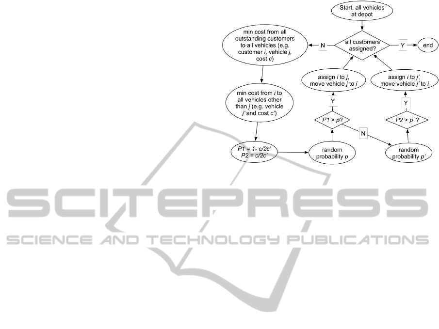
2. ﬁnd the second smallest cost from i to all vehicles,

record vehicle number j

, and cost c

3. for j, accept customer i with probability P

= 1 −

c/2c

and reject i with probability 1 − P

, so that

the smaller c is compared to c

, the bigger chance

j will be selected to serve i. On the other hand if

c = c

, or the costs of using j and j

are equivalent,

the probability becomes 1/2;

4. if customer rejected in 3), it is then assigned to

vehicle j

with probability P

= c/2d

5. if the customer is assigned to neither vehicles, the

process restarts, and in the immediate next itera-

tion, i will not be considered for selection to avoid

repeating the same situation; otherwise, move the

chosen vehicle to i and go to 1).

This approach has certain resemblance to the greedy

heuristic, because priority is always given to the as-

signment with the smallest arc cost. In every stage

of the algorithm, we keep track of the cumulative ser-

vice time of each vehicle, and returns a vehicle to the

depot if no more assignment is possible.

Each iteration of the algorithm takes very little

time, so we can run it many times and keep the best

solution. We will provide empirical studies in Section

4. We also emphasize that this is an approach that can

be implemented fairly easily, and does not require the

use of an underlying MIP solver, thus has great value

for many small ﬂeet managers with limited resources

for sophisticated implementations.

Nonetheless, the randomized approach clearly

runs the risk of sub-optimal solutions. In particular,

the number of feasible routes is exponentially large,

with only a small fraction of these being generated in

the randomized runs. This therefore motivates us to

consider a hybrid approach, blending the route-based

approach with an underlying MIP structure for com-

bining routes effectively, with the aim of being able to

ﬁnd higher-quality solutions when more sophisticated

implementations are viable.

3.3 Route Based Formulation

In some cases, when more time is allowed to ﬁnd

good solutions and more sophisticated technology is

available, we can expand our idea to leverage the

strength of an optimization-based approach, and take

advantage of the randomized approach to reduce the

problem size and improve tractability. We present the

route-based model (also referred to as the composite

variable model (Armacost et al., 2002; Barlatt et al.,

2009)). We need the following additional notations:

• R

: set of possible routes of customers that can be

served by a vehicle of type t;

Figure 1: Flow chart for the greedy heuristic.

• w

: binary variable that equals 1 if and only if

route r ∈ R

is served by a vehicle of type t ∈ T ; 0

otherwise

• C

: cost associated with assigning route r ∈ R

a vehicle of type t ∈ T

• δ

: binary indicator of whether a node i ∈ N

covered by a route r ∈ R

;

The route-based model can then be formulated as

follows:

(S) minimize

∑

t∈T

∑

r∈R

subject to:

∑

t∈T

∑

r∈R

· w

= 1 i ∈ N

(7)

∑

r∈R

≤ M

t ∈ T (8)

∈ {0,1} r ∈ R

,t ∈ T

Here constraint (7) ensures that each customer is cov-

ered by one and only one route. Constraint (8) forces

the number of vehicles of each type used to be no

more than the total number of that type.

Observe that if we were to enumerate all routes,

solving this problem would lead to an optimal solu-

tion. In reality, this is impractical for all but very

small instances. Techniques such as column genera-

tion and branch-and-price (Barnhart et al., 1998) may

be applied to problems like this, and iteratively gen-

erate only routes that appear promising. However, the

problems for ﬁnding such routes are essentially VRP

type and NP-hard. In the Appendix, we show that for-

mulation (S) is stronger than (C), and it is therefore

advantageous to work with (S).

We leverage the speed of the randomized ap-

proach from Section 3.2 with the power of the route-

VEHITS2015-InternationalConferenceonVehicleTechnologyandIntelligentTransportSystems

based formulation above to improve the solution qual-

ity. First we run the randomized heuristic for a large

number of iterations. Instead of keeping only the set

of routes with the smallest cost, all routes generated

in each iteration are put into a pool of routes. Once

the route generation is ﬁnished, we will have many

candidate routes that are cost efﬁcient. Then we for-

mulate problem (S) with the poll of candidate routes,

and solve it to ﬁnd the best route combination.

4 RESULTS AND DISCUSSION

4.1 Baseline — Genetic Algorithm

In order to provide a comparison for the proposed

algorithm against an existing class of algorithms, a

genetic algorithm (GA) (Holland, 1975) was devel-

oped. GA is suitable for a wide range of combinato-

rial problems, including VRP. Recent applications of

the GA to various VRP problems have shown its com-

petitiveness with other heuristic techniques in both

computation time and quality (Baker and Ayechew,

2003). Our implementation of the GA is based on the

“pure GA” described in Baker and Ayechew (Baker

and Ayechew, 2003). In this approach, the problem is

decomposed into two steps. The ﬁrst, controlled by

the GA, assigns customers to individual vehicles and

over time moves the solution space to be less infea-

sible and lower in cost. Since this does not establish

the order in which customers assigned to a vehicle

are to be visited, a 2-opt algorithm (Lin et al., 1965)

is employed to solve the corresponding TSP for each

individual vehicle.

Our GA implementation is performed in Matlab

on a Windows 7 machine with an Intel Core i5-

2520M processor at 2.5GHz and 8GB RAM. In or-

der to test the quality of the developed algorithm, sev-

eral test datasets were chosen from branchandcut.org,

themselves cases from published articles. The results

for these experiments, with the alphanumeric naming

convention given, are shown in Table 1. Moreover, we

considered one more dataset that was extracted from

the actual daily service routes of a food-gathering

company. We randomly selected ﬁve of their exist-

ing routes (spanning 58 customers) as well as the ve-

hicles serving these routes, calculated the travel time

between each pair of locations and compiled this into

a travel-time matrix. To obtain cost information, we

used average costs per mile for each individual ve-

hicle (this information can be obtained by multiply-

ing the fuel consumption per mile and corresponding

fuel price. One of the methods for accurate fuel con-

sumption estimation is presented in Kolmanovsky et

al. (Kolmanovsky et al., 2011). We assume the maxi-

mum work time for a vehicle/driver is eight hours.

Table 1: Performance of GA solution vs. the best known

solution on test cases.

Case Best sol. GA sol. Difference

A-n37-k5 669 731.9 9.41%

E-n23-k3 569 569.7 0.13%

E-n30-k3 534 557.8 4.47%

P-n16-k8 450 451.9 0.43%

P-n55-k8 588 677.8 15.27%

58-Node N/A 187.1 N/A

4.2 The Value of Explicitly Considering

Heterogeneous Arc Costs, and Our

Heuristics Compared with the GA

In current practices, HFVRP is often solved using a

single cost across all vehicles for each arc, for ex-

ample, the minimum cost, maximum cost, or aver-

age cost. Once the routes have been constructed, they

are then assigned to individual vehicles and the true

costs of assigning vehicles to routes can be accurately

calculated. In this experiment, we consider the value

of considering the true (vehicle-speciﬁc) costs explic-

itly when designing the vehicle routes. The following

experiments were performed with c++ on a Mac Pro

with two 2.8GHz Intel Xeon CPU and 10Gb of RAM.

The food-gathering company data is a simpliﬁca-

tion that assumes Pareto dominance across vehicles –

that is, if Vehicle A is more cost-effective on one arc

than Vehicle B, then it will be more cost-effective on

all arcs. This is often not the case and, in fact, the

motivation for our research comes from cases where

this is not true. Thus, we generated three additional

instances that are not Pareto-dominant. Cost pertur-

bation was done by multiplying each entry in the cost

matrix by a random number. For slight cost pertur-

bation, the random number was uniformly taken be-

tween 0.8 and 1.2; for medium cost perturbation, the

random number was uniformly taken between 0.5 and

1.5; and for large perturbation, the random number

was uniformly taken between 0.3 and 1.7.

For each of these four instances, we solve the

HFVRP four times. In the ﬁrst, we apply the solver-

free heuristic from Section 3.2 (H1), using the aver-

age cost data (i.e., for each arc, we take the average

across all vehicle types for that arc). After construct-

ing the routes, we then assign them to speciﬁc vehi-

cles: the most fuel-efﬁcient vehicle gets the longest

route, the second most fuel-efﬁcient vehicle gets the

AlgorithmsfortheHybridFleetVehicleRoutingProblem

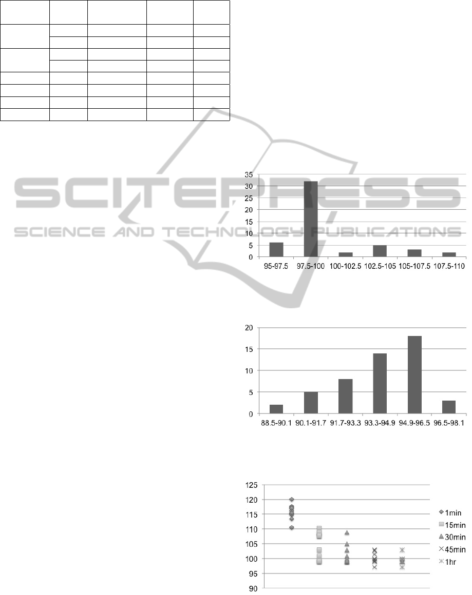
Table 2: Absolute and relative costs of solutions from dif-

ferent cost structure between VRP and HFVRP.

Pareto Low None- Medium High

Pareto

H1 with 150 152 153 122

avg. cost 104% 107% 124% 132%

H1 with 149 145 126 95

true cost 103% 102% 103% 103%

H2 with 146 145 142 123

avg. cost 101% 102% 116% 133%

H2 with 145 142 123 93

true cost 100% 100% 100% 100%

second longest route, etc. Fuel efﬁciency is measured

by average fuel cost across all arcs. Finally, we com-

pute the ﬁnal cost using each vehicles speciﬁc arc

costs. In the second approach, we apply Heuristic 1

using the true arc costs within the heuristic. In both

of these two approaches, we set a one-hour time limit

on run time. In the third approach, we use the solver-

based heuristic from Section 3.3 (H2) with the aver-

age cost data. In the fourth, we use the true cost data.

For both solver-based heuristic runs, we use 100,000

randomly generated columns.

Results appear in Table 2. Observe that in all four

instances, for either heuristic, incorporating true costs

in the initial route construction reduces cost (by as

much as 33% in one instance). This shows that, with

the same algorithm, explicitly considering the cost of

individual vehicles provides an advantage over using

an uniform cost for all vehicles in the route generation

process. Moreover, Heuristic 2 always achieves bet-

ter solutions compared with Heuristic 1 on the same

datasets, which is no surprise given the much larger

set of routes available for selection in the set partition-

ing model. Furthermore, compared to results in Table

1, all four implementations of our heuristics outper-

formed the GA, sometimes by as much as 22%.

It is not surprising that the additional value of ap-

plying our approaches improves as the data becomes

less Pareto-dominant. We therefore focus on the most

highly non-Pareto instance for the remainder of our

computational experiments.

4.3 The Effect of Randomness/heuristic

Parameters on Performance

Because our two heuristics both have signiﬁcant ran-

dom components, we next test to see the variation in

outcomes.

Returning to the complete data set (again with the

least-Pareto dominant arc costs), we apply solver-free

Heuristic 1 ﬁfty times using a run time limit of one

hour for each run. Figure 2 shows the variation in ob-

jective value. Note the limited range in solution val-

ues. We repeat the previous experiment using solver-

based Heuristic 2 with a limit of 100,000 columns.

Results appear in the Figure 3.

Recognizing that the solution quality of the

heuristics depends in part on the algorithmic param-

eters, we conduct the following experiments: we run

the solver-free heuristic with ﬁve different time limits:

1 minute, 15 minutes, 30 minutes, 45 minutes, and 60

minutes. For each time limit, we run ten random in-

stances of the heuristic. Results are displayed in Fig-

ure 4. Observe that increased runtime improves per-

formance both in reducing objective value and varia-

tion between individual tests.

Figure 2: Histogram of objective values from 50 runs of

heuristic 1 using true cost.

Figure 3: Histogram of objective values from 50 runs of

heuristic 2 using true cost.

Figure 4: Objective values from heuristic 1 under different

time limits, 10 runs for each instance.

VEHITS2015-InternationalConferenceonVehicleTechnologyandIntelligentTransportSystems

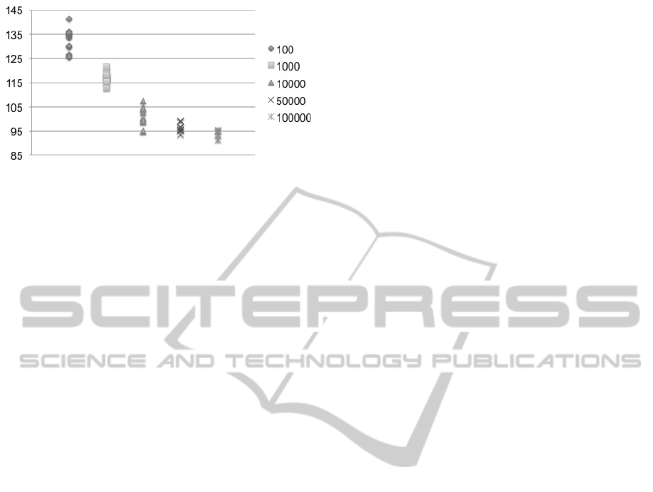
Figure 5: Objective values from Heuristic 2, with different

number of starting routes, 10 runs for each instance.

Finally, we run the solver-based heuristic with 100,

1,000, 10,000, 50,000, and 100,000 columns. For

each column limit, we run ten random instances of the

heuristic. Results are displayed in Figure 5. Clearly,

there is beneﬁt in increasing the number of columns,

with both minimum value, the average value, and the

variance all decreasing as the number of columns in-

creases.

5 CONCLUSIONS AND FUTURE

RESEARCH

Variations in vehicle type and efﬁciency are found

in virtually every vehicle ﬂeet in operations. With

the current push towards more fuel-efﬁcient and

environmentally-friendly vehicles, even greater vari-

ations are being observed, as ﬂeet operators are grad-

ually replacing older vehicles with new vehicles that

that vary substantially from the original ﬂeet compo-

sition.

Even the homogeneous-ﬂeet version of VRP is of-

ten a difﬁcult problem to solve in practice, and heuris-

tics must be employed to ﬁnd high-quality solutions

quickly. We have observed that many of the heuristic

approaches used in traditional VRP (which are often

focused on minimizing total distance traveled within

the solution) are not well-suited to HFVRP, where ex-

plicitly considering the differences in the cost struc-

ture and matching vehicle types to driving condi-

tions is critical (especially when no one vehicle type

demonstrates Pareto dominance over all the others).

We have therefore identiﬁed, implemented, and

analyzed three different approaches to gain insight

into solving this challenging and important real-world

problem. We start with an exact approach; not sur-

prisingly, this approach is only tractable for prob-

lem instances of very limited size or special struc-

ture. We next consider a greedy approach that can

quickly and easily be implemented, as well as hav-

ing very fast run times. This approach shows great

promise for those environments in which the time

to solve problem instances is limited, as are the re-

sources and IT/optimization capabilities of the ﬂeet

manager. Finally, we extend this randomized ap-

proach into a hybrid heuristic that incorporates the

randomization within an optimization-based frame-

work, typically leading to higher-quality solutions

without a signiﬁcant increase in run-time. Both of

our heuristic approaches outperformed the genetic al-

gorithm in solving a real-world HFVRP problem in

our experiments.

This research is only an initial foray into the study

of this complex problem. Several promising avenues

of investigation remain. The ﬁrst is to replace the

randomization component of the route-based prob-

lem with an optimization-based column generation

routine, where the subproblems are solved with spe-

cialized VRP algorithms (this is also referred to as

price-and-branch). The second is to extend HFVRP to

some of the other characteristics commonly observed

in real-world applications of VRP such as time win-

dows and capacity constraints. Finally, we observe

that VRPs are typically assumed to be additive – i.e.

the cost of a route is simply the sum of the individual

costs of the arcs comprising that route. In the case

of certain vehicle types, this assumption is not realis-

tic. Consider a vehicle that picks up different loads at

different locations, as the loads accumulate the mass

of the vehicle and correspondingly fuel consumption

change, which depends on the arcs traversed thus far.

We thus propose to investigate a variation of HFVRP

in which the cost of traversing a route may be non-

additive relative to the individual arc costs.

ACKNOWLEDGEMENTS

This research was supported by the National Science

Foundation under Grant SBIR-I 1013832.

REFERENCES

Armacost, A., Barnhart, C., , and Ware, K. (2002). Compos-

ite variable formulations for express shipment service

network design. Transportation Science, 35(1).

Baker, B. and Ayechew, M. (2003). A genetic algorithm for

the vehicle routing problem. Computers & Operations

Research, 30(5):787–800.

Baldacci, R., Bartolini, E., and Laporte, G. (2010). Some

applications of the generalized vehicle routing prob-

lem. Journal of the Operational Research Society,

61:1072–1077.

AlgorithmsfortheHybridFleetVehicleRoutingProblem

Baldacci, R., Battarra, M., and Vigo, D. (2008). Routing

a heterogeneous ﬂeet of vehicles. The Vehicle Rout-

ing Problem: Latest Advances and New Challenges,

43:3–27.

Baldacci, R. and Mingozzi, A. (2009). A uniﬁed exact

method for solving different classes of vehicle rout-

ing problems. Mathematical Programming, Series A,

(120):347–380.

Barlatt, A., Cohn, A., Fradkin, Y., Gusikhin, O., and Mor-

ford, C. (2009). Using composite variable modeling

to achieve realism and tractability in production plan-

ning: An example from automotive stamping. IIE

Transactions, 41(5):421–436.

Barnhart, C., Johnson, E. L., Nemhauser, G. L., Savels-

bergh, M. W., and Vance, P. H. (1998). Branch-and-

price: Column generation for solving huge integer

programs. Operations research, 46(3):316–329.

Campos, V. and Mota, E. (2000). Heuristic procedures for

the capacitated vehicle routing problem. Computa-

tional Optimization and Applications, 16:265–277.

Choi, E. and Tcha, D.-W. (2007). A column generation ap-

proach to the heterogeneous ﬂeet vehicle routing prob-

lem. Computers and Operations Research, 34:2080–

2095.

Clark, G. and Wright, J. W. (1964). Scheduling of vehicles

from a central depot to a number of delivery points.

Operations Research, 12(4):568–581.

Dantzig, G. B. and Ramser, J. H. (1959). The truck dis-

patching problem. Management Science, 6(1):80.

de Oliveira, H. C. B. and Vasconcelos, G. C. (2010). A

hybrid search method for the vehicle routing problem

with time windows. Ann Oper Res, 180:125–144.

Desrochers, M. and Verhoog, T. W. (1991). A new heuris-

tic for the ﬂeet size and mix vehicle routing problem.

Computers and Operations Research, 18(3):263–274.

Golden, B., Addad, A., Levy, L., and Gheysens, F. (1984).

The ﬂeet size and mix vehicle routing problem. Com-

puters and Operations Research, 11(1):49–66.

Gusikhin, O., MacNeille, P., and Cohn, A. (2010). Vehicle

routing to minimize mixed-ﬂeet fuel consumption and

environmental impact. In Proceedings of 7th Interna-

tional Conference on Informatics in Control, Automa-

tion and Robotics, volume 1, pages 285–291, Funchal,

Madeira -Portugal.

Hasle, G. and Kloster, O. (2007). Industrial vehicle routing.

Geometric Modelling, Numerical Simulation, and Op-

timization, pages 397–435.

Holland, J. (1975). Adaptation in natural and artiﬁcial sys-

tems, university of michigan press. Ann Arbor, MI,

1(97):5.

Kim, B.-I., Kim, S., and Sahoo, S. (2006). Waste collection

vehicle routing problem with time windows. Comput-

ers and Operations Research, 33:3624–3642.

Kolmanovsky, I., McDonough, K., and Gusikhin, O.

(2011). Estimation of fuel ﬂow for telematics-enabled

adaptive fuel and time efﬁcient vehicle routing. In

Proceeding of 11th IEEE International Conference

on Intelligent Transportation Systems Telecommuni-

cations, pages 139–144, St. Petersburg, Russia.

Kritikos, M. N. and Ioannou, G. (2010). The balanced cargo

vehicle routing problem with time windows. Interna-

tional Journal of Production Economics, 123(1):42–

51.

Laporte, G. (2009). Fifty years of vehicle routing. Trans-

portation Science, 43(4):408–416.

Li, F., Golden, B., and Wasil, E. (2007). A record-to-record

travel algorithm for solving the heterogeneous ﬂeet

vehicle routing problem. Computers and Operations

Research, 34:2734–2742.

Li, X., Tian, P., and Leung, S. C. (2010). Vehicle routing

problems with time windows and stochastic travel and

service times: models and algorithm. International

Journal of Production Economics, 125(1):137–145.

Lin, S. et al. (1965). Computer solutions of the traveling

salesman problem. Bell System Technical Journal,

44(10):2245–2269.

Novoa, C. and Storer, R. (2009). An approximate dynamic

programming approach for the vehicle routing prob-

lem with stochastic demands. European Journal of

Operations Research, 196:509–515.

Ochi, L. S., Vianna, D. S., Drummond, L. M. A., and Vic-

tor, A. O. (1998). An evolutionary hybrid metaheuris-

tic for solving the vehicle routing problem with het-

erogeneous ﬂeet. Lecture Notes in Computer Science,

1391:187–195.

Ralphs, T. K., Kopman, L., Pulleyblank, W. R., and Trot-

ter, L. E. (2003). On the capacitated vehicle routing

problem. Mathematical Programming, 94:343–359.

Salhi, S. and Rand, G. K. (1993). Incorporating vehicle

routing into the vehicle ﬂeet composition problem.

European Journal of Operations Research, 66:313–

330.

Tahmassebi, T. (1999). Vehicle routing problem (vrp)

formulation for continuous-time packing hall de-

sign/operations. Computers and Chemical Engineer-

ing Supplement, S:1011–1014.

Taillard,

E. D. (1999). A heuristic column generation

method for the heterogeneous ﬂeet vrp. Operations

Research – Recherche op

erationnelle, 33(1):1–14.

Tarantilis, C., Zachariadis, E., and Kiranoudis, C. (2008).

A guided tabu search for the heterogeneous vehicle

routing problem. Journal of the Operations Reserach

Society, 59:1659–1673.

Toth, P. and Vigo, D., editors (2001). The Vehicle Routing

Problem. Society for Industrial and Applied Mathe-

matics (SIAM).

Wassan, N. and Osman, I. (2002). Tabu serach variants for

the mix ﬂeet vehicle routing problem. Journal of the

Operations Reserach Society, 53:768–782.

APPENDIX

We denote the LP relaxation to problem (S) as (SL),

and the LP relaxation to problem (C) as (CL).

Theorem. The lower bound generated by problem

(SL) is at least as tight as the lower bound generated

by problem (CL)

VEHITS2015-InternationalConferenceonVehicleTechnologyandIntelligentTransportSystems

Proof. We ﬁrst show that, for any feasible solution

to (SL), there is a corresponding feasible solution to

(CL) with the same objective function value. For

any feasible solution, say ˆw, to problem (SL), let

ˆx

i j

∑

r∈R

ˆw

. It is easy to see that (1) and (2) are

satisﬁed since (7) and (8) are. Moreover, this solution

also satisﬁes (3), since each route r ∈ R

already guar-

antees the ﬂow conservation constraint (3) for all its

nodes. Assuming the connection costs are additive,

the objective function value corresponding to ˆx will

equal the objective value for ˆw. To see that this so-

lution also satisﬁes (6), ﬁrst note that since any route

in (SL) satisﬁes this constraint, the maximum num-

ber of legs a route r can overlap with a MVP p is

− 1. Therefore along the direction of r, there will

be at least one leg on p, either right before the start or

after the end point of the overlapping section or both,

that is exposed (i.e., not covered by r). Because of

(7), the sum of the ﬂow on the exposed leg is at most

1 − ˆw

. The sum of all “lost” ﬂows on all exposed

legs along p is therefore ≥

∑

r∈R

ˆw

≥ 1. The right

inequality holds whenever at least one vehicle of type

t is used. We can show that (4) is satisﬁed by ˆx in a

similar way.

To complete the second half of this proof, we

show that not all solutions to (SL) are feasible to (CL).

Consider a simple problem with 3 customers besides

the depot and 3 vehicles of the same type. Assuming

that the trip length limit is large enough, a solution

to (CL) can make a round-trip between each pair of

customers with “half” a vehicle (i.e., the weight of

the connection is 0.5 for both legs of the trip). This

solution will satisfy all the constraints in (CL), but

will not have a corresponding solution in (SL) since it

skips the depot altogether.

AlgorithmsfortheHybridFleetVehicleRoutingProblem