Automated Mapping of Business Process Execution Language to

Diagnostics Models

Hamza Ghandorh

and Hanan Lutﬁyya

Department of Electrical and Computer Engineering, Western University, London, Ontario, Canada

Department of Computer Science, Western University, London, Ontario, Canada

Keywords:

Web Service Composition Diagnosis, Codebook Technique, BPMN Mapping.

Abstract:

This paper illustrates how a speciﬁcation of a business process can be automatically mapped to a fault diag-

nostic model. Observed failures at run-time are quickly analyzied through the diagnostic model to determine

the faulty service.

1 INTRODUCTION

Web services are loosely-coupled, self-contained,

and self-describing modules that perform a pre-

determined task. Services can be used in multiple

applications and thus are reusable. A service of a

particular type can be replaced by another service if

necessary. The architectural paradigm for organiz-

ing distributed applications based on a composition

of web services, which may be under different own-

ership, is referred to as a Service-Oriented Architec-

ture (SOA) (Papazoglou and Van Den Heuvel, 2007) .

These compositions can be used to implement a busi-

ness processes (Lins et al., 2012).

A fault (Garza et al., 2007, Alam, 2009) is a defect

in either hardware or software that causes a failure. A

failure occurs when a service deviates from expected

behaviour. To illustrate the relationship between fault

and failure consider the following example. A hard-

ware power loss causes a service to become unavail-

able. The cause of the hardware power loss is the fault

and the failure is that the service has become unavail-

able. In another example an unexpected load may re-

sult in a service provider in not providing a response

in the expected time i.e., a Quality of Service (QoS)

requirement may be violated. The cause of the unex-

pected load is the fault and the failure is the violation

of the QoS requirement.

A fault (or problem) may cause multiple failures

(often referred to as symptoms). For example, a com-

position of services could have service WS

that com-

municates with W S

and W S

communicates with

W S

. If WS

becomes unavailable then W S

may not

be able to complete a request from W S

and thus W S

observes a failure of W S

. Another example can be

seen in a composition which consists of services W S

W S

, W S

and W S

. The ﬁrst three of these services

are clients of WS

. If the machine that W S

is hosted

on goes down (and thus W S

is not available) then the

other services observe a failure of W S

. Fault diagno-

sis is used to determine a fault and often includes anal-

ysis of notiﬁcations of failures (referred to as events).

To provide a robust service experience, it is im-

portant to have an effective and efﬁcient mechanism

for fault diagnosis (Zhang et al., 2012a). Model-based

fault diagnosis performs fault diagnosis through mod-

els. Some of these, e.g., codebook, have been shown

to be effective in practice. Many fault diagnosis mod-

els require knowledge of the application conﬁgura-

tion. With the sheer number of possible applications

there is a need to automate the development of a fault

diagnosis model.

This paper proposes an approach to the generation

of a fault diagnosis model based on a notational rep-

resentation of a business process. We show the fault

diagnosis model can be used in the management of

service compositions.

This paper is organized as follows: Section 2 pro-

vides the background, Section 3 presents related work

on fault diagnosis, Section 4 presents the proposed ap-

proach. Section 5 describes the architecture of man-

agement system for a diagnostic module that uses our

approach, Section 6 describes the results of the test-

ing of our implementation, and Section 7 concludes

the paper.

251

Ghandorh H. and Lutﬁyya H..

Automated Mapping of Business Process Execution Language to Diagnostics Models.

DOI: 10.5220/0005430702510259

In Proceedings of the 5th International Conference on Cloud Computing and Services Science (CLOSER-2015), pages 251-259

ISBN: 978-989-758-104-5

 2015 SCITEPRESS (Science and Technology Publications, Lda.)

2 BACKGROUND

This section describes fault diagnosis and a notation

for describing a business process.

2.1 Fault Diagnosis

The process of fault diagnosis requires the following:

fault detection, fault localization, and testing (Stein-

der and Sethi, 2004). Fault detection is the process

of capturing symptoms (Hanemann, 2007). Detec-

tion techniques can be based on active schemes (e.g,

polling to determine availability) and/or symptom-

based schemes, where a system component indicates

that it has detected a failure. Examples of proposed

fault detection techniques can be found in Angeli et

al (Angeli and Chatzinikolaou, 2004) and Hwang et

al (Hwang et al., 2010).

Fault localization typically requires an analysis of

a set of observed symptoms. The goal of fault local-

ization is to ﬁnd an explanation of the symptoms’ oc-

currence. The explanations are delivered in the form

of hypotheses. Hypotheses are statements which ex-

plain that each observed symptom is caused by one or

more designated problems. Based on these hypothe-

ses, a testing step is performed in order to determine

the actual problems through the application of a suit-

able testing mechanism (Steinder and Sethi, 2004).

There are several fault localization techniques

techniques. One of these, event correlation, attempts

to associate one symptom with another symptom in

order to infer the relationship between their occur-

rences (Tiffany, 2002). Through an examination of

these associations, a number of possible hypothe-

ses are generated that reﬂect the symptoms’ occur-

rence. There are several different types of correla-

tions, which are useful for diagnosing problems in a

network. One of these is described in 3.

In this work when we say that we are mapping

a business process speciﬁcation to a fault diagnosis

model we are speciﬁcally referring to a model that

supports fault localization.

2.2 BPMN

One standard that can be used to model business pro-

cesses is referred to as Business Process Modeling

Notation (BPMN)(Alonso et al., 2004) (Endert et al.,

2007). BPMN has several notational elements. An

activity node represents a web service. A link repre-

sents different possible ﬂows and is chosen based on

the result of the evaluation of a condition of an activ-

ity. A gateway represents decision points that repre-

sent a workﬂow’s conditions. A sequenceﬂow repre-

sents a link from a gateway node to an activity node.

A pool represents the combination of a composition

of ﬂowobjects, gateways, and sequenceﬂows. A mes-

sageﬂow describes the exchange of messages between

pools, and an event describes the start or end point of

workﬂow. A pool may have an activity ﬂowobject that

can be represented by another pool. Each pool repre-

sents a workﬂow and a business process is associated

with a set of pools. An example of a business pro-

cesses workﬂow modelled as a BPMN speciﬁcation

is presented in Figure 1.

3 RELATED WORK

Steinder et al. (Steinder and Sethi, 2004) proposed a

classiﬁcation of fault localization techniques which is

derived from graph-theoretic techniques and included

techniques such as codebook, context-free grammar,

and bipartite causality approaches. Graph-theoretic

techniques rely on the use of graphs. The graphs in-

clude nodes that represent symptoms and problems,

while directed edges are used to model the relation-

ship between the problems and symptoms. Essen-

tially edges represent cause-effect relationships be-

tween problems and symptoms or symptoms and

other symptoms. An example is seen in Figure 3(a).

To create such a model, an accurate knowledge of cur-

rent dependencies among the system components is

required. The rest of this section brieﬂy describes

representative work on fault diagnosis based on the

relationships between problems and symptoms.

Tighe et al. (Tighe and Bauer, 2010) imple-

mented a distributed fault diagnosis algorithm, pro-

posed by Peng and Reggia and is referred to as Par-

simonious Covering Theory (Peng and Reggia, 1990),

in a policy-based management tool called BEAT (Best

Effort Autonomic Tool) (Bahati et al., 2007). The al-

gorithm is concerned with the generation of plausi-

ble hypotheses or covers, based on given information

that comes from graph-theoretic models, prior to di-

agnosis. Hypotheses are delivered and grouped in or-

der to generate disorder-and-manifestation statements

that are forwarded to a decision making system for re-

covery actions.

Zhang et al. (Zhang et al., 2012b) proposed a

hybrid diagnosis method to diagnose web services’

problems in service-oriented architectures. Their

method combines dependency matrix-based diagno-

sis and a Bayesian network-based diagnosis. Al-

though the authors considered the reduction of the

computational complexity of services diagnosis, the

hybrid diagnosis method does not cope with the dy-

namic nature of SOA’s services, and Bayesian net-

CLOSER2015-5thInternationalConferenceonCloudComputingandServicesScience

252

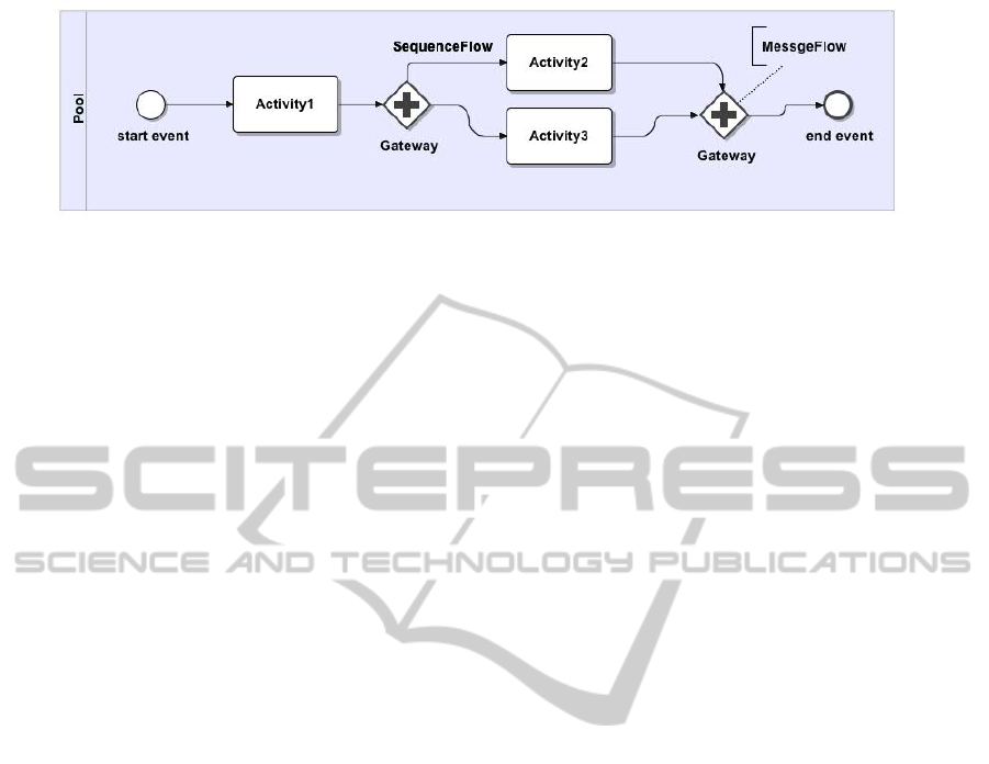
Figure 1: Simple BPMN example.

work diagnosis provides slow measurement.

Ardissono et al. (Ardissono et al., n.d.) proposed a

model-based diagnostic framework with autonomous

diagnostic capabilities to monitor the state of web ser-

vices. As a partially distributed approach, the frame-

work includes several local diagnosers, which is at-

tached to a web service or a composition, cooperate

with a global diagnostic service. As soon as local di-

agnosers notice a problem, they raise an alarm to the

global diagnostic service to detect it.

Most of the above work focuses on the models.

None of the work investigated shows how to automate

the development of a fault diagnosis model based on a

speciﬁcation of a business process. However, there is

work (e.g., (Mor

an et al., 2011)) that takes a business

process speciﬁcation and maps it to control rules.

4 PROPOSED APPROACH

This section describes our approach to using the

BPMN speciﬁcation of a business process to a fault

diagnosis model.

4.1 Codebook Technique

Earlier we discussed that a fault may manifest itself in

the unexpected behaviour of a web service that is ob-

served by other web services. For our our fault diag-

nosis model we use a fault propagation model, which

describes which symptoms that may be observed if a

speciﬁc fault occurs (K

atker and Paterok, 1997). The

underlying mathematical structure is typically a graph

(Steinder and Sethi, 2004). For this work we chose the

codebook technique (Kliger et al., 1995). This tech-

nique was implemented in a network fault diagnostic

system and the results (Yemini et al., 1996) suggest

that this approach is highly scalable.

The codebook technique or coding technique

(Steinder and Sethi, 2004) uses a causality graph and

problem code (PC) matrix of a web service compo-

sition’s workﬂow to locate the source of failures. A

causality graph is a bipartite graph whose vertices can

be partitioned into two disjoint subsets V and W such

that each edge connects a vertex from V to one from

W (Caldwell, 1995). A PC matrix is a matrix repre-

sentation of a causality graph used to infer the causes

of observed symptoms. The PC matrix is built based

on the causality graph. An example of the causality

graph and the matrix are illustrated in Figure 3(a) and

3(b), respectively. The matrix consists of a column

that represents symptoms that problems cause. A ma-

trix entry either has the value of zero or one. For ex-

ample, the value of one assigned at PC [1, 1] position

in PC matrix indicates that symptom S

can be ob-

served for problem P

. The value of zero assigned at

PC[1, 3] position indicates that symptom S

can not

be observed for problem P

At run-time a problem will cause one or more

symptoms to be generated. From this a string can be

formulated. If the i

symptom was observed then the

position in the string is one otherwise it is zero.

This string will be referred to as a current symptoms

vector (CSV).

The diagnosis process uses the Hamming dis-

tance. The Hamming distance is the minimum num-

ber of substitutions that transforms one string into the

another. For example, the Hamming distance between

two words “toned” and “roses” is three letters and the

Hamming distance between the two strings 1011101

and 1001001 is two bits (MacKay, 2005). Each value

in a column in the PC matrix is compared with its

corresponding code in a given CSV. If both values are

identical (i.e, the value in the column in the PC ma-

trix and its corresponding code in the given CSV are

the same), the Hamming distance value is denoted as

zero. Otherwise, the Hamming distance is denoted

as one. The values are then summed to determine

the Hamming distance of the two words. The mini-

mum of the Hamming distance values is an indicator

of the corresponding problems as the causative prob-

lems. For the PC matrix, if the given CSV is 11000,

the Hamming distance is (0,4,4) for columns labeled

and P

respectively. Thus, the causative prob-

lem was P

. If the given CSV is 11101, the Hamming

distance is (2,2,4) for columns labeled P

, P

and P

Thus, the causative problems are limited to P

and P

AutomatedMappingofBusinessProcessExecutionLanguagetoDiagnosticsModels

253

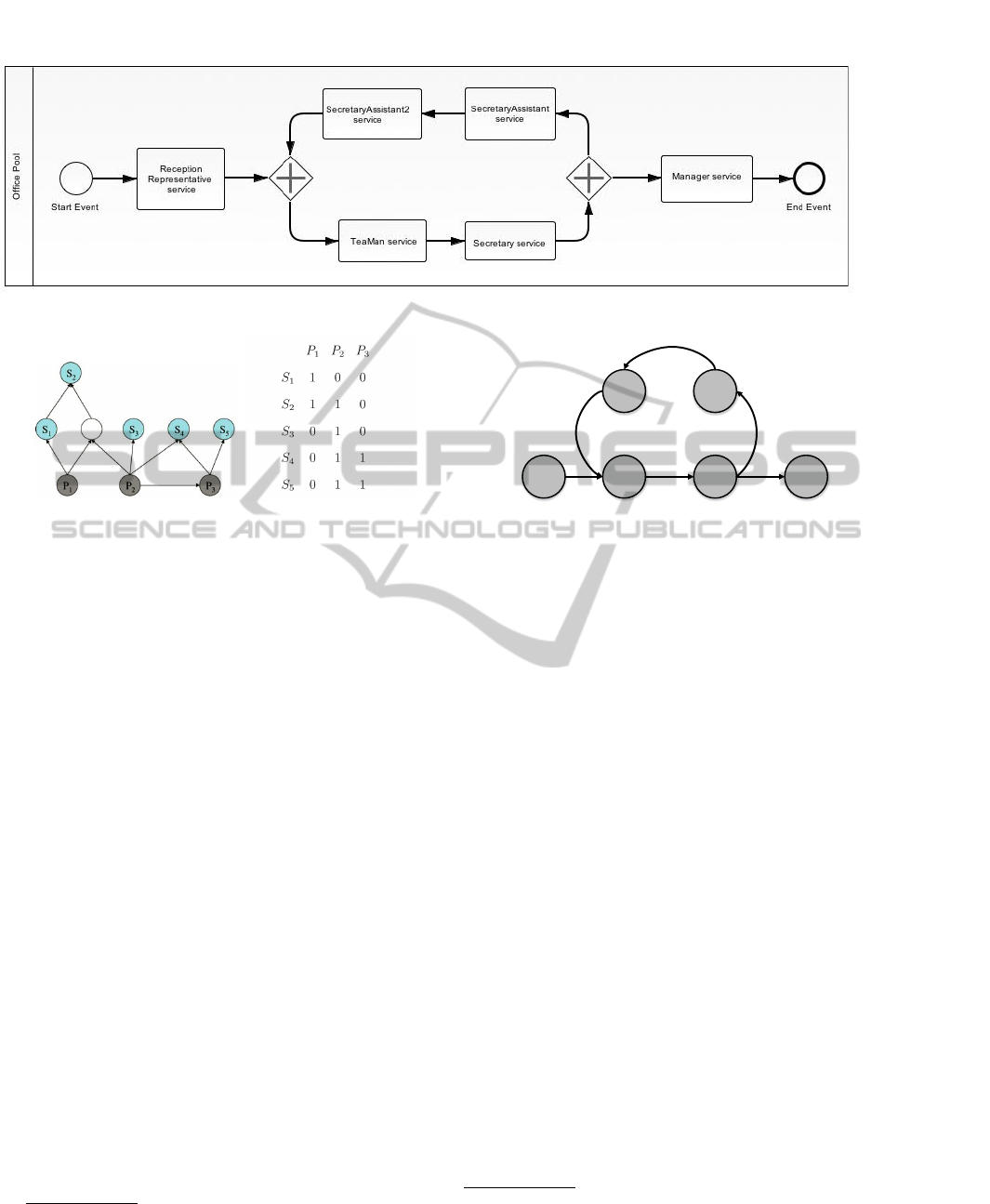
Figure 2: Ofﬁce Business Process BPMN.

(a) Causality Graph (b) PC matrix

Figure 3: Example of causality graph and PC matrix (Stein-

der and Sethi, 2004).

4.2 BPMN Mapping

The BPMN mapping is done through the transforma-

tion from BPMN graphs to a composition dependency

(CD) graph which is done prior to determining the

causality graph. For illustration purposes, Figure 2

presents BPMN model for a ofﬁce business process,

which is concerned with delivering only important

mails to the manager ofﬁce through different ﬁlters.

The transformation from BPMN to a CD graph is per-

formed as follows: assume that a CD graph is repre-

sented as (V ,E). Each BPMN atomic activity node is

a node in V . If a decision point follows an activity

then the node in V representing the activity will have

two outgoing edges. Edges represent different possi-

ble ﬂows. Figure 4 depicts the CD graph for the ofﬁce

business process, where P

represents the Reception-

Representative service, P

represents the TeaMan ser-

vice, P

represents the Secretary service,P

represents

the SecretaryAssistant service, P

represents the Sec-

retaryAssistant2 service and P

represents the Man-

ager service. We note that the granularity of the model

is limited to a service. Hence a problem, P

, corre-

sponds to a service. We will use the notation P

refer to both a problem and to a service.

Assume that the CD graph is represented as (V ,E)

while the causality graph is represented as (V

)

The causality graph vertices are known in advance

Figure 4: Abstract View of Ofﬁce Business Process.

The set V

can be partitioned into two sets W ,X such

that each edge in E

connects a vertex from W to a ver-

tex in X . The set W is the set of potential problems.

Since each node in the CD graph represents an activ-

ity and any of these activities can be faulty then the set

of W is the same as the set V . Let v be a node in a CD

graph. This node represents a potential problem. Any

node, u, in the CD graph, for which there exists a path

from it to the node v, potentially could exhibit a fail-

ure condition if v becomes faulty. Any node that could

exhibit a failure condition is in set X. For a node u we

use the notation P

to represent u as a problem and S

to represent u as a symptom. Determining the causal-

ity graph of the CD graph requires these two algo-

rithms: Modiﬁed Deph-ﬁrst Search (mdfs), and path-

Generator. The mdfs and pathGenerator algorithms

are presented in algorithm 1 and algorithm 2, respec-

tively. The mdfs algorithm takes as input a CD graph

and does a depth-ﬁrst traversal. When all child nodes

of node v have been traversed then the pathGenera-

tor algorithm is used to generate all paths from node

v to each leaf node. These paths are used to produce

the causality graph. The causality graph of the ofﬁce

business process is depicted in Figure 5.

The mdfs algorithm uses two variables: Vertices-

List, and BackTrackEdgesList. VerticesList is a list

that keeps track of each node’s label. The Back-

TrackEdgesList maintains a list of backtrack edges.

A backtrack edge (v,w) indicates that the mdfs algo-

based on the given information from a client about fault and

symptom quantities

CLOSER2015-5thInternationalConferenceonCloudComputingandServicesScience

254

Figure 5: Causality graph of the ofﬁce business process.

rithm is revisiting node w and that not all of node w’s

children had yet been visited. White is a label that

indicates an unvisited node, which is the initial state

for all nodes. Gray is a label that indicates a node

has been visited but not all of its children have been

traversed. Black is a label that indicates a node has

been visited and all of its children have been pro-

cessed. When the input CD graph is received, mdfs

is triggered (line 1). If the current node being visited

is White, mdfs will assign the Gray label (line 3). The

mdfs algorithm examines each outgoing edge (lines 4-

5). If the node on the other end of the edge is labelled

White then this means that the node has not been vis-

ited and thus no paths have been generated (lines 6-

7). If the node on the other end of the edge is labelled

Gray then the edge is put in the BackTrackEdgesList

(lines 8-9). If there is no unvisited neighbour node for

the current node, mdfs executes the pathGenerator al-

gorithm in order to generate paths (line 12).

The pathGenerator algorithm is executed when all

nodes on the other end of the outgoing edges of node v

have been visited. The pathGenerator uses three vari-

ables: newPath, pathsW, and Paths. The newPath

variable is used to represent a sequence of nodes, and

pathsW represents a set that contains all the paths

from w to all leaf nodes. Paths is a container for all

possible paths. The pathGenerator algorithm is exe-

cuted when a current node v is received from mdfs.

The pathGenerator looks for outgoing edges of node

v. If there are no outgoing edges (line 2), the path-

Generator algorithm creates a new path, appends v

node in this path, and adds the path to Paths (lines

5-7). If there are one or many outgoing edges (line 8),

the pathGenerator algorithm retrieves each path asso-

ciated with w and creates a new path by putting to-

gether v and the path associated with w (lines 10-19).

The execution of the algorithms does not always

provide all paths. This happens where there is a cy-

cle. The existence of backtrack edges indicate a cy-

cle. Assume a backtrack edge: (v,w). The mdfs algo-

rithm will generate all paths from node w to leaf nodes

but the paths generated for node v will not include

those paths that start at w. For example, the edge

) is a backtrack edge in Figure 4. The paths

from the root node (P

) to all nodes in the ofﬁce CD

graph are: ((P

) , (P

, P

) , (P

, P

) , (P

, P

) ,

, P

) ,(P

, P

)) . After considering

the backtrack edge (P

) , the paths will be: ((P

) ,

, P

) , (P

, P

) , (P

, P

)

, (P

, P

) , (P

, P

)) . Paths

generated considering backtrack edges are done after

mdfs terminates. Let (v,w) be a backtrack node. Let

P be the set of paths. For each path that ends with w

create a new path that appends v to the path that ends

with w.

Algorithm 1: Modiﬁed depth-ﬁrst search(mdfs).

Procedure: mdfs executed on receipt Graph G

with root node v

Input : G = (V, E) where

E =

{

(v, w)|v, w ∈ V

}

and node v is

a zero indegree edge and all nodes

v are initially unvisited.

Variables : VerticesList carrys on all nodes,

White is label for unvisited node

state, Gray is label for the visited

but not ﬁnished node state. Black is

label for the ﬁnished node state.

BackTrackEdgesList carrys on

edges resulted from visiting Gray

nodes.

1 mdfs(G,v)

2 if VerticesList [v] = White then

3 VerticesList [v] = Gray

4 forall the e ∈ G.incidentEdges(v) do

5 w = G.incidentEdges(v, e)

6 if VerticesList [w] = White then

7 mdfs(G, w)

8 else if VerticesList [v] =Gray then

9 putEdge(v,w,BackTrackEdgesList)

10 VerticesList [v] = Black

11 // when there are zero unvisited

nodes, backtrack

12 pathGenerator(v)

4.3 Diagnostic Models

The Codebook technique (Steinder and Sethi, 2004)

is used as our diagnostic model. Each path generated

starts from a node v and ends at a node w. If a problem

occurs in node w then it is possible that symptoms are

detected by each node in the path. Thus each path

generated is represented in PC matrix as a column.

We see this with Figure 5 and Table 1.

AutomatedMappingofBusinessProcessExecutionLanguagetoDiagnosticsModels

255

Algorithm 2: pathGenerator.

Procedure: pathGenerator executed on receipt

a graph G and node v

Input : Graph G and node v from mdfs

Variables : newPath, pathsW, and Paths

Output : Possible set of paths

1 begin

2 if G.incidentEdges(v) == null then

3 // Create a new path, add v

node in this path, and add the

path to Paths

4 newPath = null

5 newPath.append(v)

6 Paths = Paths ∪ newPath

7 else

8 forall the e ∈ G.incidentEdges(v) do

9 w = G.incidentEdges(v, e)

10 pathsW = emptySet

11 // Retrieve all previously

generated paths from w to

each leaf node reachable

from w

12 forall the p ∈ Paths.get(w) do

13 newPath = null

14 newPath.append(v)

15 newPath.append(p)

16 pathsW.add(p)

17 Paths = Paths ∪ pathsW

Table 1: Problem codes matrix for the ofﬁce business pro-

cess.

S1 1 1 1 1 1 1 1

S2 0 1 1 1 1 1 1

S3 0 0 1 1 1 1 1

S4 0 0 1 0 1 1 0

S5 0 0 1 0 0 1 0

S6 0 0 0 0 0 0 1

By apply the mdfs and pathGenerator algorithms

on the ofﬁce CD graph, in Figure 5, since S4 can be

observed for P

, the PC[4, 4] is assigned the value of

one. Since symptom S5 can not be observed for P

PC[5, 6] has been assigned the value 0. All codes as-

signed to present the causality relationships in Fig-

ure 5 are portrayed in table 1. In table 1, there are two

columns representing different patterns that result in

symptoms associated with the web service that is as-

sociated with problem P

. These are represented by

, P

Fault diagnosis assumes a vector of symptoms that

have been reported. It is assumed that these symp-

toms are generated by a failure detection component

located within a composition. The Hamming dis-

tance between the vector and each column is calcu-

lated. The lower the value of the Hamming distance

the more likely that the column explains what is caus-

ing the symptoms.

For the ofﬁce business process assume that the fol-

lowing symptoms are observed: P

says that P

has

timed out, P

says that P

has timed out, P

says that

has timed out, and P

says that P

has timed out,

and P

says that P

is not responding. For this pat-

tern of symptoms, the CSV is 111110. Based on the

PC matrix for the ofﬁce business process, the result

list is depicted at Table 2. From Table 2, the causative

web service for the observed symptoms are P

and

since they have the minimum values between their

peers.

Table 2: Result list of the ofﬁce business process.

S1 0 0 0 0 0 0 0

S2 1 0 0 0 0 0 0

S3 1 1 0 0 0 0 0

S4 1 1 0 1 0 0 1

S5 1 1 0 1 1 0 1

S6 0 0 0 0 0 0 1

∑

4 3 0 2 1 0 3

5 ARCHITECTURE

Section 4 presents an approach to automating the de-

velopment of a fault diagnostic model. This model

is part of the diagnosis module of a third party

third party policy-based management system (Hasan,

2011). The management system allows for Service-

Level Agreements (SLAs) to be negotiated. These

SLAs formalize the QoS requirements. Policies are

used for three types of decisions: service selection,

SLA violation and recovery policies (Hasan, 2011).

The service selection policy is deﬁned by clients to

guide choice of services. The violation policy speci-

ﬁes what constitutes a violation of an SLA. The recov-

ery policy is deﬁned by clients that speciﬁes recovery

actions to be taken when the management system de-

tects a SLA violation.

5.1 TPA

A key component in the management system is the

third party agent (TPA). The TPA carries out these

tasks: (1) allows all clients, providers, and provided

services to be registered with it; (2) negotiates SLAs,

CLOSER2015-5thInternationalConferenceonCloudComputingandServicesScience

256

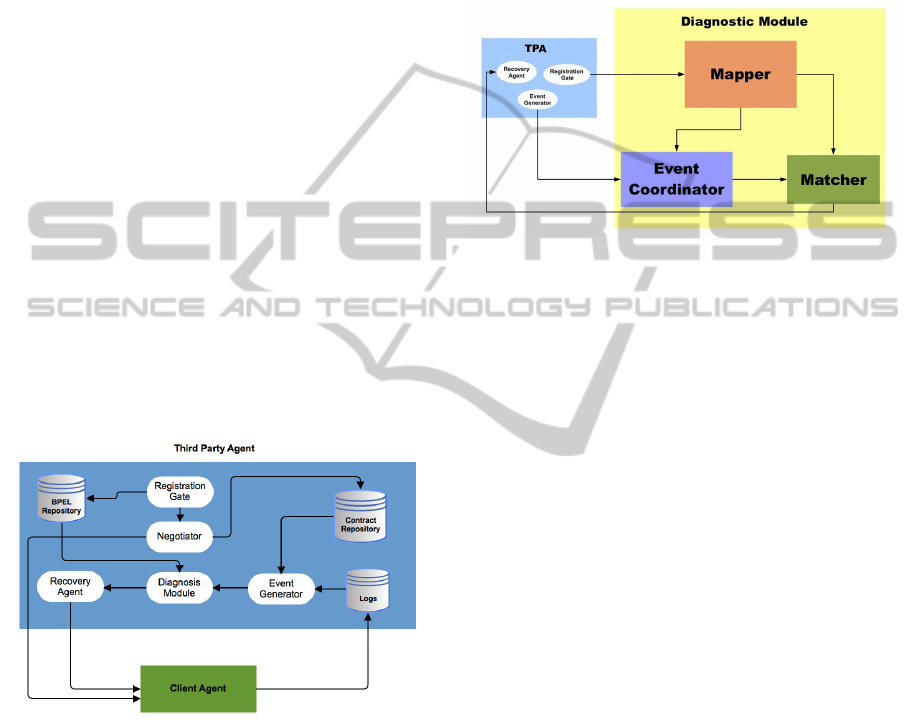
polices, and keeps track of violated SLAs; (3) gen-

erates events to indicate failures and performs recov-

ery actions. An overview of the TPA is presented as

Figure 6. The Registration Gate is responsible for

(1) forwarding a business process speciﬁcation to the

BPMN Repository, which stores the BPMN speciﬁ-

cation for each composition being managed by the

TPA. This is one of the inputs for the Diagnosis Mod-

ule. (2) forwarding relevant information about clients

and providers to the Negotiator. The Negotiator is re-

sponsible for maintaining an agreement (i.e. SLA)

between a client and a service provider if both parties

have a match between the former’s needs and the lat-

ter’s speciﬁcation. These agreements are stored in the

Contract Repository. The Event Generator relies on

the stored information found in logs storage, such as,

information related to service invocations. The Event

Generator also “uses SLAs and SLA violation poli-

cies to generate events that represent SLA violations

... when the number [SLA violations] exceeds what

is speciﬁed in the SLA violation policy then an event

is generated”(Hasan, 2011). The diagnosis module

receives the generated events and uses the generated

diagnosic model to deliver a diagnostic hypotheses.

The Recovery Agent is responsible for analysing the

diagnosis module’s hypotheses and executing reactive

actions.

Figure 6: TPA with the Client Agent.

5.2 Diagnosis Module Overview

Our proposed diagnosis module provides a hypothe-

sis about the source of symptoms observed in a com-

position. The basic module architecture is presented

in Figure 7. There are main three components: (1)

The Mapper which transforms received BPMN spec-

iﬁcations to PC matrix; (2) The Event Coordinator

which transforms the generated events to CSV; (3)

The Matcher which is responsible for matching PC

matrix and CSV to deliver a hypothesis to the Recov-

ery Agent. The Mapper is only used for new appli-

cations or if an application is modiﬁed. Otherwise at

run-time only the Event Coordinator and Matcher are

used. We note that our model narrows the problem to

a service. Further tests could be carried out to further

narrow down the root cause. However, for recovery

purposes it may be sufﬁcient to know the service that

is causing failures and the action could be to select

another instance of the same type.

Figure 7: Diagnosis module with the TPA.

6 EVALUATION

After we implemented the Mapper, the Event Coor-

dinator, and the Matcher components, we tested our

diagnosis module on composition description graphs

to see if the module is able to accurately and correctly

determine the source of events. We ran the diagno-

sis module on a single machine with 2.66 GHz In-

tel Core 2 Duo processor, Mac OS X 10.6.8 , and

eight gigabyte 1.07 GHz memory. We used Netbeans

7.0.1 IDE to run tests and create or manipulate CSVs.

For the transformation from BPMN to the composi-

tion description graphs, we used a tool referred to as

the BPMN Modeler, which is an extension of eclipse

IDE (Eclipse, 2011). The BPMN Modeler is respon-

sible for creating a BPMN for a business process and

forwarding a BPMN textual description to the Map-

per component.

We applied our diagnosis module to nine subjects

which consists of: single or many joins (i.e. sin-

gle or many vertices’ edges ending in one vertex),

single or many splits (i.e. single or many vertices’

edges starting from one vertex and ending at an other

vertex), single or many cycles (i.e. single or many

vertices’ edges starting and ending at the same ver-

tex), self cycles (i.e. single vertex’ edges is starting

and ending at the same vertex), and trees (i.e. single

or more vertices are interconnected in a hierarchical

manner). For each performed test, we assumed that

one fault could happen for each subject. For each sub-

ject we did a test for each web service going down.

All evaluation results and speciﬁcations and execu-

AutomatedMappingofBusinessProcessExecutionLanguagetoDiagnosticsModels

257

Table 3: Nine CD graphs speciﬁcations.

Graph

Vertices

Number

Edges

Number

Single

Cycle

Self

Cycle

Many

Cycles

Single

Split

Many

Splits

Single

Join

Many

Joins

Diagnosis

Time

Execution

Time

Ofﬁce

6 6 • • • 3.2 1.68

2 CD 1 7 9 • • 5.8 1.85

3 CD 2 6 6 • 2 1.65

4 CD 3 10 10 • • 13.2 2.24

5 CD 4 11 12 • • 9 2.30

6 CD 5 16 20 • • 32.8 5.87

7 CD 6 100 114 • • • 328.8 16.16

8 CD 7 9 11 • • 9.4 1.93

9 CD 8 33 34 • • • 32.8 5.43

Time measured in milliseconds

Time measured in seconds

tion time of composition dependencies graphs are pre-

sented in table 3. A correct diagnosis was found 100%

of the time. In cyclic composition description graphs,

the diagnosis module indicates not only the problem-

atic node but also the closest predecessor node to the

causative node. The reason is that both the causative

node and the predecessor node have the same code in

the PC matrix. Thus, any faults occurring in either

these nodes will generate the same events in the com-

position.

7 CONCLUSION

This paper focused on an automated mapping of a

business process speciﬁcation to a diagnostic model.

By using our diagnosis module the complexity of di-

agnosis can be hidden from system administrators by

outsourcing this functionality to a third party agent.

The proposed approach enhances the automated di-

agnosis for a large number of compositions. This

section brieﬂy discusses the work and possible future

work.

Scalability. There are two aspects to this. At run-

time there is a need to compare a set of symptoms

with each column of the problem code (PC) matrix.

There has been considerable work on making this fast

as noted in (Steinder and Sethi, 2004) and the work

on a network fault management system (Yemini et al.,

1996) shows that the use of the codebook can be very

effective at run-time. This suggests that this approach

will be scalable at run-time for service compositions.

The second aspect is the generation of the PC ma-

trix. This requires two algorithms: mdfs and path-

Generator. The mdfs algorithm is based on a modiﬁed

depth-ﬁrst search algorithm. Although compositions

may be large, it is unlikely they will be so large that

it would not be feasible to run the algorithms. We

note that the generation of the PC matrix only needs

to be done once for a speciﬁc composition. If a web

service is replaced by another web service there is no

need to generate a new PC matrix. If the composition

changes then a new PC matrix needs to be generated.

However, as future work will look at reusing part of

the computation of the PC matrix for an older version

of the application in order to reduce the time to create

a new PC Matrix if the application topology changes.

Granularity. The granularity of the diagnosis

model is limited to each service. If a service is con-

sidered to be a problem then a set of tests needs to be

carried out to investigate why the service is a problem

e.g., is the host down; is the service down. Further-

more it may be possible to use information in error

messages to improve the granularity. This will be a

topic of investigation for further studies. However, we

note that for recovery purposes the level of granularity

may often be satisfactory. If a service often violates

its SLA then it may feasible to replace it with another

service of the same type. The reasons for SLA viola-

tion are not necessarily relevant.

Mappings. This work considered only mapping

from a BPMN model to a codebook fault diagnosis

model. Further work will look at other businesses

processes speciﬁcations as well as other fault diag-

nostic approaches. The current version of the diag-

nosis module only uses the the codebook technique.

Since the coding phase is performed only once, the

codebook approach is very fast, robust, and efﬁcient.

However, the accuracy of the codebook technique is

hard to predict when more than one problem occurs

with overlapping sets of symptoms. In addition, since

each change of system conﬁgurations requires regen-

erating the codebook, the technique is not suitable for

environments with dynamically changing dependen-

cies (Steinder and Sethi, 2004). We will enable the

module to use several event correlations techniques

CLOSER2015-5thInternationalConferenceonCloudComputingandServicesScience

258

by which the module will be able to regenerate more

efﬁcient diagnostic knowledge bases.

ACKNOWLEDGEMENTS

The research for this paper was ﬁnancially supported

by the Ministry of Education of Saudi Arabia, and

College of Computer Science and Engineering at

Taibah University

and the Natural Sciences and En-

gineering Research Council of Canada (NSERC).

REFERENCES

Alam, S. (2009), Fault management of web services, Mas-

ter, University of Saskatchewan.

Alonso, G., Casati, F., Kuno, H. and Machiraju, V. (2004),

Web Services: Concepts, Architectures and Applica-

tions, 1st edition edn, Springer.

Angeli, C. and Chatzinikolaou, A. (2004), ‘Online fault de-

tection techniques for technical systems: A survey’,

International Journal of Computer Science and Ap-

plications 1, 51–64.

Ardissono, L., Console, L., Goy, A., Petrone, G., Picardi,

C. and Segnan, M. (n.d.), ‘Towards self-diagnosing

web services’, http://citeseerx.ist.psu.edu/viewdoc/

summary?doi=10.1.1.75.1874.

Bahati, R. M., Bauer, M. A. and Vieira, E. M.

(2007), Policy-driven autonomic management of

multi-component systems, in ‘Proceedings of 2007

the conference of the center for advanced studies on

Collaborative research’, ACM, pp. 137–151.

Caldwell, C. (1995), ‘Graph Theory Glossary’,

http://www.utm.edu/departments/math/graph/

glossary.html#b. Online; accessed 05-June-2011.

Eclipse (2011), ‘BPMN Modeler’, http://eclipse.org/bpmn/.

Online; accessed 17-Oct-2011.

Endert, H., Hirsch, B., K

uster, T. and Albayrak, S. (2007),

Towards a mapping from bpmn to agents, Proceedings

of the 2007 international workshop and 2007 confer-

ence on Service-oriented computing: agents, seman-

tics, and engineering, Springer-Verlag, Berlin, Heidel-

berg, pp. 92–106.

Garza, A., Serrano, J., Carot, R. and Valdez, J. (2007), Mod-

eling and simulation by petri networks of a fault toler-

ant agent node, in ‘Analysis and Design of Intelligent

Systems using Soft Computing Techniques’, Vol. 41

of Advances in Soft Computing, Springer Berlin / Hei-

delberg, pp. 707–716.

Hanemann, A. (2007), Automated IT Service Fault Diag-

nosis Based on Event Correlation Techniques, PhD

thesis, LMU Mnchen: Faculty of Mathematics, Com-

puter Science and Statistics.

Taibah University site https://www.taibahu.edu.sa/

Pages/AR/Home.aspx

Hasan, M. S. (2011), Policy Based Third Party Web Service

Management, Master, University of Western Ontario.

Hwang, I., Kim, S., Kim, Y. and Seah (2010), ‘A survey

of fault detection, isolation, and reconﬁguration meth-

ods’, Control Systems Technology, IEEE Transactions

on 18(3), 636–653.

atker, S. and Paterok, M. (1997), Fault isolation and event

correlation for integrated fault management, in ‘Inte-

grated Network Management V’, Springer, pp. 583–

596.

Kliger, S., Yemini, S., Yemini, Y., Ohsie, D. and Stolfo,

S. (1995), A coding approach to event correlation,

in ‘Integrated Network Management IV’, Springer,

pp. 266–277.

Lins, F., Damasceno, J., Souza, A., Silva, B., Arag

ao, D.,

Medeiros, R., Sousa, E. and Rosa, N. (2012), ‘To-

wards automation of soa-based business processes’,

International Journal of Computer Science, Engineer-

ing and Applications 2(2), 1–17.

MacKay, D. J. (2005), Binary codes, in ‘Information The-

ory, Inference & Learning Algorithms’, Cambridge

University Press, pp. 206–227.

Mor

an, D., Vaquero, L. M. and Gal

an, F. (2011), Elasti-

cally ruling the cloud: specifying application’s be-

havior in federated clouds, in ‘Cloud Computing

(CLOUD), 2011 IEEE International Conference on’,

IEEE, pp. 89–96.

Papazoglou, M. P. and Van Den Heuvel, W.-J. (2007), ‘Ser-

vice oriented architectures: approaches, technologies

and research issues’, The VLDB journal 16(3), 389–

415.

Peng, Y. and Reggia, J. A. (1990), Abductive inference mod-

els for diagnostic problem-solving, Springer-Verlag

New York, Inc.

Steinder, M. and Sethi, A. S. (2004), ‘A survey of fault lo-

calization techniques in computer networks’, Science

of Computer Programming 53(2), 165–194.

Tiffany, M. (2002), ‘A Survey of Event Correlation

Techniques and Related Topics’, http://citeseerx.

ist.psu.edu/viewdoc/summary?doi=10.1.1.19.5339.

Online; accessed 19-Dec-2010.

Tighe, M. and Bauer, M. (2010), Mapping policies to a

causal network for diagnosis, in ‘6th International

Conference on Autonomic and Autonomous Sys-

tems’, pp. 13–19.

Yemini, S. A., Kliger, S., Mozes, E., Yemini, Y. and Ohsie,

D. (1996), ‘High speed and robust event correlation’,

Communications Magazine, IEEE 34(5), 82–90.

Zhang, J., Huang, Z. and Lin, K.-J. (2012a), A hybrid

diagnosis approach for qos management in service-

oriented architecture, in ‘Web Services (ICWS),

2012 IEEE 19th International Conference on’, IEEE,

pp. 82–89.

Zhang, J., Huang, Z. and Lin, K.-J. (2012b), A hybrid

diagnosis approach for qos management in service-

oriented architecture, in ‘19th IEEE International

Conference on Web Services’, pp. 82–89.

AutomatedMappingofBusinessProcessExecutionLanguagetoDiagnosticsModels

259