Central Model Predictive Control of a Group of Domestic Heat Pumps

Case Study for a Small District

R. P. van Leeuwen

1,2

, J. Fink

and G. J. M. Smit

Department of Computer Science, Mathematics and Electrical Engineering, University of Twente,

P.O. Box 217, 7500 AE Enschede, The Netherlands

Sustainable Energy Group, Saxion University of Applied Sciences, P.O. Box 70.000, 7500 KB Enschede, The Netherlands

Keywords:

Heat Pump, Smart Grid Control, Domestic Hot Water, Floor Heating, Thermal Storage, Model Predictive

Control, Optimization.

Abstract:

In this paper we investigate optimal control of a group of heat pumps. Each heat pump provides space heating

and domestic hot water to a single household. Besides a heat pump, each house has a buffer for domestic hot

water and a ﬂoor heating system for space heating. The paper describes models and algorithms used for the

prediction and planning steps in order to obtain a planning for the heat pumps. The optimization algorithm

minimizes the maximum peak electricity demand of the district. Simulated results demonstrate the resulting

aggregated electricity demand, the obtained thermal comfort and the state of charge of the domestic hot water

storage for an example house. Our results show that a model predictive control outperforms conventional

control of individual heat pumps based on feedback control principles.

1 INTRODUCTION

In the Netherlands, approximately 40% of the total

domestic energy consumption is related to space heat-

ing and domestic hot water (ECN, 2014). To this date,

most Dutch houses rely on natural gas supply and gas

boilers. Heat pumps powered by renewable electric

energy are a possible way to make the transition to-

wards integration of renewable energy in the build-

ing environment (Janssen-Visschers and Lee, 2013),

(Scheepers et al., 2007). In the small city Meppel,

a new district is under construction with an almost

100% renewable energy supply (Meppelenergie, ND).

A biogas CHP provides heat for houses connected to

district heating and electric power for other houses

with a heat pump. Imports and exports of electric en-

ergy from and to the national grid are possible, but the

heat pumps should use the electricity from the CHP

as much as possible. Development of a smart grid

control system is the joined task of a project group

formed by University of Twente, University of Delft,

the utility Rendo, Meppel city council and system in-

tegrator i-NRG.

The Meppel case explores local sustainability, not

only due to the employed energy system, but also due

to the legal aspects. The entire district heating and

cooling system including the heat pumps which are

placed at some of the houses, are owned by a utility

company which is founded speciﬁcally for this dis-

trict. Only the supply of hot water for space heating

and domestic hot water is sold by the utility company

to the households, either delivered by the district heat-

ing system, or the heat pumps. The utility company

is not allowed to supply households electricity for do-

mestic appliances, e.g. TV’s and washing machines.

Hence, electric power supply to the heat pumps is

through a separated cable. As a consequence, it is

possible that the utility company controls starting and

stopping of each heat pump on a central level.

Our previous paper (Fink et al., 2014) was aimed

at developing a mathematical approach to solve the

large scale central optimization problem in an efﬁ-

cient way. In that paper solving one big instance

of MILP (Mixed Integer Linear Program) for every

time step of 15 minutes is compared with a more efﬁ-

cient method called time scale MILP. However, a pre-

calculated data table is used for the prediction of heat

demand of 100 households. With this table, the rela-

tion between the heat pump planning and the achieved

thermal comfort within the households cannot be in-

vestigated. In this paper, model predictive control re-

places the pre-calculated data table.

Main contributions of this paper are: describing

a method for model predictive control for planning

136

van Leeuwen R., Fink J. and J. M. Smit G..

Central Model Predictive Control of a Group of Domestic Heat Pumps - Case Study for a Small District.

DOI: 10.5220/0005434301360147

In Proceedings of the 4th International Conference on Smart Cities and Green ICT Systems (SMARTGREENS-2015), pages 136-147

ISBN: 978-989-758-105-2

 2015 SCITEPRESS (Science and Technology Publications, Lda.)

of heat pumps in a district, demonstrating the qual-

ity of the heat pump planning for minimizing the

peak electricity consumption and demonstrating the

achievable thermal comfort within the households.

Furthermore, comparing this result with conventional

feedback control of individual heat pumps.

The paper is structured as follows. Section 2 con-

siders related work to heat pump planning in smart

micro grids and model predictive control. In Section

3, models are formulated for prediction of space heat-

ing and domestic hot water demand and input data for

the Meppel case is described. Section 4 formulates

the general control and optimization problem. Sec-

tion 5 shows results on the achievable aggregated en-

ergy consumption proﬁle of the heat pumps. Also, the

resulting thermal comfort of the households is shown.

Finally, conclusions are given in Section 6, including

a discussion on future work.

2 RELATED WORK

Planning of electric devices in micro-grids is a re-

cent investigation area. In this paper, Triana, a multi-

commodity and optimization tool is employed. Dif-

ferent forms of energy (e.g. electricity, heat, biogas)

can be simulated in relation to a single optimization

objective. Triana is developed at the University of

Twente, the Netherlands.

To obtain ﬂexibility within a smart grid, it is re-

quired that (a) devices are controllable or (b) the func-

tion of the device can be shifted in time without un-

acceptable consequences for the customer. Such de-

vices are batteries, (dish)washing machines, dryers,

fridges and heat pumps. (Bosman, 2012) developed

speciﬁc planning algorithms for smart micro grids,

while (Bakker, 2011) and (Molderink et al., 2010) in-

vestigate various case applications like the planning

of a group of fridges in relation to varying electric-

ity price schemes, due to renewable energy produc-

tion by solar PV. (Claessen et al., 2014) compare two

smart grid control approaches, i.e. Triana and Intel-

ligator. The Triana approach contains three steps to

control devices: prediction on the device level, plan-

ning based on price signals from the aggregator and

real time control by the device controller. The Intelli-

gator approach is based on the Powermatcher concept

(Kok et al., 2005) which uses a multi-agent electric-

ity market. Device agents send bids to a central auc-

tioneer agent. The price signal from the auctioneer

clears the market with the purpose to adjust the bids

in such a way that the market equilibrium (and con-

sumption) is steered towards the optimization objec-

tive. Claessen demonstrates that both approaches are

able to reach certain objectives but also demonstrates

the improvement which is possible when predictions

are part of the approach.

In this paper, the Triana approach without market

based steering principles is applied. In the Meppel

case it is possible to simplify the control method and

let a central controller directly determine the planning

of the heat pumps based on heat demand predictions

for each household. Hence, the planning and real time

control steps are basically the same. The planning

step considers planning of the heat pumps from 2 up

to 24 hours ahead, whereas the real time control step

considers planning of the heat pumps for the actual

time up to 1 or 2 hours ahead. This approach leads

to a method called ”time scale MILP” in (Fink et al.,

2014). The central controller has to solve one large

optimization problem every time step of 15 minutes

with a time window of 24 hours ahead. However, the

size of the problem is reduced by considering larger

time steps for moments further in time. In this way,

the planning is more and more approximated, the fur-

ther it looks into the future.

A heat pump is an electric appliance with a low

temperature thermal input and higher temperature

thermal output which is used for space heating or do-

mestic hot water (Mitchel and Braun, 2013), (Hep-

basli and Kalinci, 2009). Model predictive control

(MPC) of heat pumps in the building environment is

a recent investigation area. MPC is investigated ei-

ther for building climate control to minimize energy

consumption, or for power balancing of smart micro

grids. Early work on MPC for building climate con-

trol is performed by Madsen et al (Madsen and Holst,

1995). Recent investigations which include experi-

mental results are carried out by (Oldewurtel et al.,

2012), (

Sirok

y et al., 2011) and (Pr

ıvara et al., 2011).

(Halvgaard et al., 2012) investigates the use of MPC

for the control of a domestic heat pump in relation

to minimizing energy costs for heating a house, for

which Nordic spot market electricity prices are taken

as input data. (Dar et al., 2014) demonstrates how a

domestic heat pump can be controlled by MPC such

that self consumption of PV-generated electricity is

increased.

The previously mentioned research on MPC con-

siders climate control of single buildings with em-

phasis on the quality of model predictions and the

quality of reaching the objectives, i.e. minimizing

costs or energy consumption. Based on this work,

the conclusion is justiﬁed that MPC is a promising

control method which outperforms conventional feed-

back control methods when the control system has

more objectives than room temperature control. Our

main interest, however, is not on the optimal control

CentralModelPredictiveControlofaGroupofDomesticHeatPumps-CaseStudyforaSmallDistrict

137

of a single building or heat pump, but the application

of MPC to control many houses with heat pumps in

a district. The main goal and contribution of this pa-

per is to demonstrate the quality of reaching multiple

objectives for a smart micro grid with MPC controlled

heat pumps, i.e. minimizing peak loads on the electric

network, maintaining thermal comfort in the houses

and adequate charge states of domestic hot water stor-

ages.

3 PREDICTIVE MODELS

3.1 Model of the Energy System

In Figure 1, a schematic overview of the energy sys-

tem is given. The picture shows a range of houses

(labeled 1 to n, in which n is the number of houses).

Each house has a heat pump (HP) which is connected

to two types of thermal buffers: (a) a ﬂoor heating

system and (b) a hot water storage for domestic hot

water (DHW). The ability of the ﬂoor heating to store

thermal energy and possible consequences on thermal

comfort and costs is demonstrated in (Leeuwen et al.,

2014). The energy inputs to the heat pumps are: (a)

low temperature source energy from an underground

thermal storage and (b) electric energy from a biogas

Combined Heat and Power system (CHP), which due

to the constant biogas ﬂow runs continuously. The

CHP is also connected to the main electricity grid.

Heat produced by the CHP is distributed via a large,

centrally located thermal storage to a district heating

network which involves much more houses than the

number of houses with a heat pump.

This energy system is a combination and further

development of two common types of local renew-

able energy systems: district heating based on bio-

gas co-generation and heat pumps combined with un-

derground thermal storage. In the Netherlands, Ger-

many and Denmark there are numerous regional ar-

eas where biogas from waste water treatment plants is

used as a source for co-generation of heat and power

which is distributed to local consumers through a dis-

trict heating network and a local electricity grid which

has a connection to the larger grid. A large scale ex-

ample of this is Apeldoorn Zuidbroek (Dreijerink and

Uitzinger, 2013) where 2500 houses are heated in this

way.

An aquifer underground thermal storage is used as

a source for cooling and for heat pumps. An aquifer

is an underground groundwater reservoir at a depth of

around 60-120 meters. The temperature of the wa-

ter is around 15

◦

C, which is used as source energy

for heat pump evaporators during the heating sea-

Figure 1: Schematic picture of the energy system.

son. During the summer, the groundwater is used

to cool the houses, which also regenerates the reser-

voir temperature after the heat pumps have cooled the

reservoir down during the heating season. In recent

years, this type of storage is commonly applied for

new larger buildings and urban areas in North West-

ern Europe. The increasing use of heat pumps in new

building projects combined with suitable soil condi-

tions and existence of large underground aquifers al-

most anywhere in the Netherlands, result in increas-

ing applications of this type of storage.

In general, the purpose of the energy system is

to provide the new district with almost 100% renew-

able energy for heating and cooling of houses. As

the energy system is a combination of existing op-

tions which are proven in practice, more cases with

a similar energy system are expected to be developed

in the future.

The energy system is conﬁgured in such a way that

the average electric production of the CHP equals the

average required electric input by all heat pumps on

the coldest possible day. Furthermore, there are only

two energy prices, arranged by contract with the grid

operator. A low price for selling electricity from the

CHP to the grid and a high price for buying electricity

from the grid. Hence, the objectives for the heat pump

control are:

• maintain thermal comfort for space heating within

each house

• maintain sufﬁcient state of charge of the hot water

buffer to cover DHW demand of each house

• use electricity of the CHP as much as possi-

ble locally for the heat pumps and avoid buying

electricity from the grid. This objective can be

reached when the electric demand is ﬂattened to-

wards the average. Also, investments in electric-

ity cables throughout the district and transformers

at the energy house are minimal when the peak

electric demand is as low as possible. Therefore,

the control objective is formulated as: minimize

SMARTGREENS2015-4thInternationalConferenceonSmartCitiesandGreenICTSystems

138

Figure 2: 2R2C model.

peaks of the aggregated heat pump electricity de-

mand.

Following the area plan of the Meppel building

project, 104 houses with a heat pump are studied. At

this stage, the houses involved are not yet built and

hence, the study involves simulations based on spe-

ciﬁc models which are discussed in the following sub-

sections.

3.2 Household Space Heating Demand

Model

In (Fink et al., 2014), a data table per house is used as

predictive information for the space heating demand.

However, a data table should be based on relevant re-

lations between space heating demand and inﬂuences

such as weather conditions or occupancy. For this,

a simulation model can be used or an online model

which learns relations from measurement data. With-

out a model as integral part of the control system,

it is impossible to estimate the consequences on the

thermal comfort when storage ﬂexibility of the house

structure (thermal mass) is exploited to optimize the

control. Applying a model instead of a data table

has the advantage that temperatures which are rele-

vant for people’s comfort are pre-calculated during

the planning phase and deviations with real-time mea-

surements can be corrected during an online real-time

control phase. Therefore, a model is used to predict

space heating demand for each house in this paper.

For the model of space heating demand in relation

to ambient conditions, the following general 2R2C

thermal network model shown in Figure 2 is adopted

which contains a thermal mass term (C

) for the ﬂoor

heating and internal zone of the house (C

). The

model contains the following parameters (Table 1):

The generalized model equation is given by:

= AT + Bq (1)

In which the vector T contains the thermal mass and

ambient temperatures and vector q contains direct

heat gains to or loss terms from the thermal masses,

Table 1: Model parameters.

resistance between ﬂoor heating and zone

capacitance of ﬂoor heating

thermal resistance of house envelope

capacitance of the zone

window area on each side of the building

solar energy on building planes with windows

heating energy injected into ﬂoor heating

gain

thermal gains by occupants and appliances

vent

heat loss by ventilation air ﬂow

in f

heat loss by inﬁltration air ﬂow

i.e. heating input to the ﬂoor heating and solar en-

ergy gains to the zone. Matrix A characterizes sys-

tem dynamics and contains thermal capacitance and

resistance parameters. Matrix B speciﬁes how the di-

rect heat gains and losses enter the respective thermal

masses.

Model parameters are estimated for 4 types of ref-

erence houses (AgentschapNL, 2013) for which sim-

ulated response data is generated in TRNSYS (TESS,

ND). The accuracy of this approach is investigated in

detail in (Leeuwen et al., 2015). The parameters for

the 4 house types are given in Table 2 in which: TH-

Terraced House, CH-Corner House, SDH-Semi De-

tached House, DH-Detached House.

Table 2: Estimated 2R2C model parameters.

unit TH CH SDH DH

K/kW 3.26 2.81 1.69 1.66

kWh/K 3.61 3.61 4.56 5.08

K/kW 11.01 8.23 8.67 7.17

kWh/K 10.62 16.74 20.34 22.48

The window areas for each building plane are

given in (AgentschapNL, 2013). Effective solar trans-

mission through the window into the house is calcu-

lated by multiplying the window area of each building

plane with the incident total radiation on the plane

and a transmission factor. The houses are oriented

according to the district area plan into the 4 major

wind directions. Incident total solar radiation on each

building plane is calculated from measured horizontal

total radiation, i.e. from weather station Hoogeveen

of the Royal Dutch weather institute, which is near

to the city of Meppel. The calculation of diffuse

and beam radiation is based on theory outlined in

(Dufﬁe and Beckman, 1980). To calculate the amount

of diffuse radiation from total horizontal radiation

measurements, a correlation proposed in (Erbs et al.,

1982) is used.

In total, there are 104 houses. At present, the pos-

sible types of occupancy (families, couples, etc.) in

relation to the types of houses is not known. Based

on a comparative study of a recent built district in

CentralModelPredictiveControlofaGroupofDomesticHeatPumps-CaseStudyforaSmallDistrict

139

the Netherlands (Blokker and Poortema, 2007), the

following 3 types of occupancy and distribution over

104 households are deﬁned: young family (52%), el-

der couple (15%) and young couple (33%). For the

house orientation, indicated by the facing direction

of the front facade, and the distribution of occupant

types over the different house types, the following is

listed, in which the relation between occupant type

and house orientation is assumed to be random:

• 41 terraced houses with the following number of

houses in combination with the front plane direc-

tion: 20-North/4-East/7-South/10-West. Number

of households in combination with occupant-type:

12-young family/2-elder couple/27-young couple.

• 20 corner houses: 10-North/2-East/4-South/4-

West. Households and occupant-type: 18-young

family/0-elder couple/2-young couple.

• 26 semi detached houses: 0-North/10-East/4-

South/12-West. Households and occupant-type:

16-young family/6-elder couple/4-young couple.

• 17 detached houses: 0-North/8-East/8-South/1-

West. Households and occupant-type: 8-young

family/8-elder couple/1-young couple.

3.3 Occupancy Related Thermal Losses

or Gains

For each type of occupancy, hourly schedules are de-

ﬁned for working days and days of the weekend for

relevant thermal events. The schedules are related to

common behavioral patterns of working people. For

this paper, statistical backgrounds of schedules are not

investigated. For each occupancy type, basic sched-

ules are deﬁned including randomization of some of

the time points at which thermal events occur. In the

following, the basic approach for the programming in-

volved is explained. For the occupancy type: young

family, a working weekday schedule is shown in Fig-

ure 3. Further in the paper, a young family is also

considered when discussing the results. The ﬁgure

shows relative to a deﬁned maximum, the following

thermal events:

• Occupancy: thermal gains by occupants present

in the house. Schedules consist of a number of

time points at which the number of occupants

which are present in the house are deﬁned. Based

on (Mitchel and Braun, 2013) the thermal gain

by people is on average 40 W per person during

sleeping hours and 110 W per person during day

and evening hours. Figure 3 shows the number of

occupants present in the house.

• Ventilation rates: typically, ventilation schedules

depend on: (a) the time of the day, (b) the num-

ber of occupants present in the house, (c) cooking

events which require higher ventilation rates, (d)

shower or bath events in the bathroom which re-

quire higher ventilation rates. The ventilation sys-

tem has 4 states for the ventilation rate: (1) cook-

ing, (2) high, (3) medium, (4) low. This relates to

typical existing Dutch house ventilation systems.

Figure 3 shows ventilation rates for each hour.

• Appliance thermal gains: Four appliance classes

are deﬁned: (1) computers/television, (2) light-

ing, (3) fridge/freezer, (4) background appliances

like pumps, fans and standby electronic equip-

ment. The total yearly electricity consumption of

the schedule in Figure 3 is approximately equiv-

alent to Dutch average consumption ﬁgures pub-

lished by (Milieucentraal, ND).

• DHW (Domestic Hot Water) demand: for a single

household this is determined by several events at

certain timepoints each day. In total, 6 possible

events are deﬁned, each with a speciﬁc amount

of required water of 40

◦

C: (1) shower, (2) bath,

(3) hand cleaning, (4) small dish wash, (5) large

dish wash and (6) body washing. Figure 3 shows

the water amounts for a number of events. The

amount of water per event and the time points are

slightly randomized.

In the same way, schedules are worked out for other

occupancy types, both for working days and weekend

days.

3.4 Heat Pump Model

Heat pump performance is approximated as a constant

relation between electric input and thermal output of

the heat pump for two operational modes: space heat-

ing mode with an output temperature of 35

◦

C and

thermal storage mode with an output temperature of

◦

C. Hence, the heat pump has 3 operational states:

(1) off, (2) space heating, (3) thermal storage. The

relation is given in table 3 which is based on supplier

data (Alpha-Innotec, 2014).

Table 3: Heat pump energy speciﬁcation.

state unit input output

off kW 0.0 0.0

space heating kW 1.3 6.0

thermal storage kW 1.8 5.0

SMARTGREENS2015-4thInternationalConferenceonSmartCitiesandGreenICTSystems

140

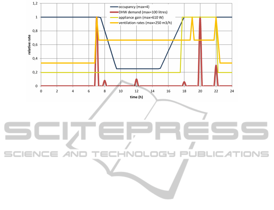
Figure 3: Example weekday thermal event schedule.

4 CONTROL ALGORITHMS

In (Fink et al., 2014) a general approach for off-

line and on-line heat pump central control problems

is introduced. This paper concerns an off-line prob-

lem because the weather and occupancy related data

are known beforehand as forecasts. The optimiza-

tion process is explained in more detail in (Fink

and Hurink, 2015). For the simulation, the predic-

tive models, house type deﬁnitions, occupant related

schedules, weather calculation module, reference and

optimization control algorithms are deﬁned as Python

script ﬁles. The Triana simulation environment, de-

veloped at the University of Twente is written in C++.

MILP instances are solved by the CPLEX solver

package.

4.1 Optimized Control

Following the Triana smart grid method, planning of

the heat pumps is determined in two calculation steps:

a prediction step and a planning step. The Triana

method also contains a third step: real time control,

but for this type of off-line problem, this step is irrel-

evant: it is assumed for now that there is no deviation

between the prediction and the simulated reality. On

the other hand, if an on-line control problem is stud-

ied, the real time control step involves a comparison

between measurements in real time and predictions

for the short term, resulting in adjustment of the short

term heat pump control planning to reduce possible

deviations.

The control objective to minimize peak electric

demand is formulated as:

Minimize max

t∈T

∑

· X

c,op,t

∈

{

0, 1

}

(2)

In which E

is the electric demand of a heat pump

converter. op ∈

{

sh, dhw

}

denotes an operational

mode of the heat pump within a set of operational

modes, in this case space heating (sh) or domestic hot

water (dhw). X

c,op,t

is the control state for each heat

pump converter.

c ∈

{

1, 2, . . . , n

}

denotes a heat pump converter

for each house within a set of heat pump converters

which totals the number of houses (n). The time in-

terval t ∈ T denotes that all time intervals t are within

the planning period T . Each heat pump is either ”on”

c,op,t

= 1) or ”off” (X

c,op,t

= 0). However, two op-

erational modes for one heat pump cannot be ”on” at

the same time, that is

∑

c,op,t

≤ 1. For this we in-

troduce additional control variables.

Let x, y and z be control states for which: x, y, z ∈

X. Let x

c,t

be the control variable for space heating

during the prediction phase, y

c,t

be the control vari-

able for space heating during the planning phase and

c,t

be the control variable for DHW during the plan-

ning phase. The ﬁrst stage heat pump planning x

c,t

for space heating is determined in the ﬁrst phase of

the calculation, i.e. the prediction phase optimizes:

Minimize

∑

c,op,t

0 ≤ X

c,op,t

≤ 1

subject to the following constraints:

• T z

≥ T

pre f ,t

for all t ∈ T where T

pre f ,t

is the set-

point operative temperature.

• the thermal load of a house is modeled with (1)

which relates the ﬂoor heating temperatures and

zone temperatures to heat losses to the ambient

and to heat gains and heat input from the heat

pumps.

• pre-calculation of occupancy related thermal

gains and ventilation losses based on schedules.

CentralModelPredictiveControlofaGroupofDomesticHeatPumps-CaseStudyforaSmallDistrict

141

• pre-calculation of solar gains.

The output of the prediction phase is a ﬁrst stage plan-

ning of the heat pumps in order to exactly match the

space heating demand of each house.

During the second phase of the calculation, i.e. the

planning phase, the ﬁrst stage planning of the space

heating converters is re-calculated but now the op-

timization includes a space heating thermal buffer.

Also, calculation of the planning now includes the

DHW demand prediction and the State of Charge of

the DHW thermal buffer. Equation (2) is now subject

to the following constraints:

• 0 ≤

∑

i=1

c,i

− x

c,i

) ≤

max

hp,sh

∆t

in which y

c,i

sig-

niﬁes the re-planned control states of each con-

verter for space heating and q

hp,sh

the thermal out-

put of the heat pump for space heating: q

hp,sh

c,sh,t

· output

c,sh

in which output

c,sh

is the ther-

mal output of the heat pump speciﬁed in Table 3.

∆t signiﬁes the incremental length of the time in-

terval t and SH

max

the maximum capacity of the

space heating buffer. This capacity is determined

in (Leeuwen et al., 2014).

• 0 ≤ SoC

≤ DHW

max

in which SoC

signiﬁes the

State of Charge of the DHW buffer and DHW

max

the maximum capacity of the DHW buffer, i.e. de-

termined by the water volume and fully charged

average temperature.

• SoC

t+1

= SoC

+ z

c,t

· q

hp,dhw

− D

t,dhw

which

yields the control states of the heat pump convert-

ers z

c,t

for the DHW operation mode. q

hp,dwh

sig-

niﬁes the heat pump thermal output and D

t,dhw

the

DHW demand during time period t. Heat loss of

the heat buffer is not modeled, but could be incor-

porated in D

t,dhw

4.2 Reference Control

The reference control is based on a simple set of feed-

back control rules which results in approximately the

same behavior as individual PID control of each heat

pump. At each time interval, the following is evalu-

ated for each house:

• For space heating, the operative temperature T z

is compared with T

pre f ,t

which is the minimum

allowed temperature deﬁned in schedules. If the

operative temperature is below this value, the heat

pump is on. If it is above this value plus a positive

deadband value, the heat pump is off.

• For DHW, the State of Charge of the buffer SoC

is compared with a minimum allowed value. If

the SoC is below this value, the heat pump is on.

If it is above a value close to the maximum SoC,

the heat pump is off.

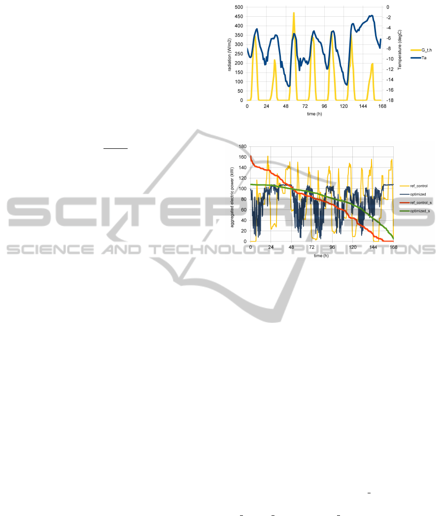
Figure 4: Input weather data.

Figure 5: Aggregated electrical energy demand.

• Operation of the heat pump for DHW has priority

over space heating: y

c,t

= 0 if z

c,t

= 1.

5 CASE STUDY RESULTS

5.1 Results for a Cold Week

To discuss the quality of the obtained results, the cold-

est week of the year 2012 is investigated ﬁrst. This

week has the highest average heat demand and there-

fore the longest peak load duration is expected during

this week. The input weather data, i.e. the ambient

temperature (Ta) and global horizontal solar radiation

t,h

) are shown in Figure 4.

In Figure 5 the electrical energy demand is

shown for the reference control (ref control) and op-

timized control. The sorted values from high to low

(ref control s and optimized s) demonstrate the qual-

ity of the peak minimization by the optimized con-

trol. The peak for the reference control is 162 kW.

This is the peak electric consumption when all heat

pumps have their own on/off controlled thermostats.

The peak for the optimized control is 108 kW. The

average electricity power for the shown period is 74

kW. Compared to this average, the maximum peak of

the reference control is 119% higher and of the opti-

mized control 46% higher.

SMARTGREENS2015-4thInternationalConferenceonSmartCitiesandGreenICTSystems

142

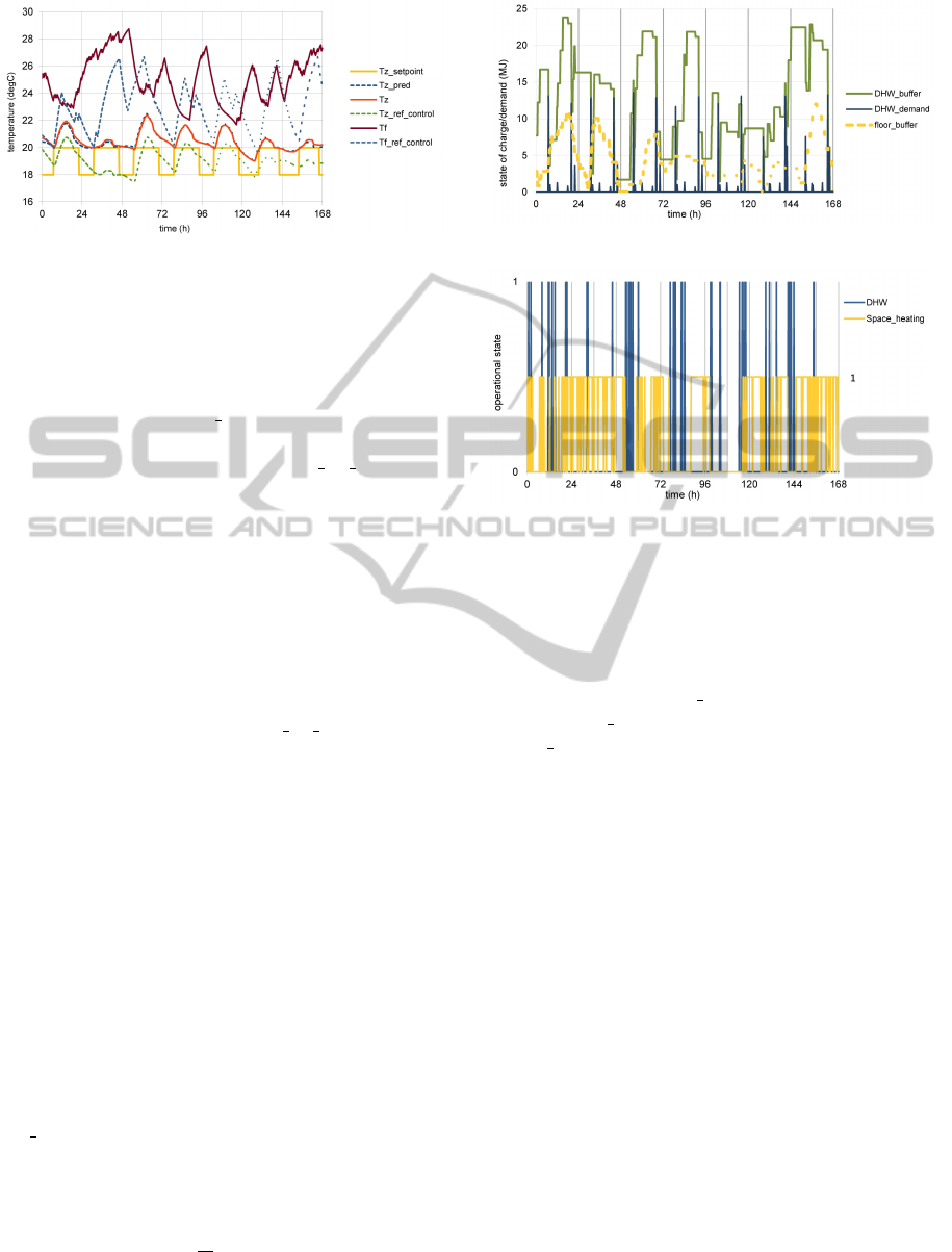
Figure 6: Example indoor operative and ﬂoor heating tem-

peratures.

Figure 6 shows an example of the indoor operative

and ﬂoor heating temperatures for the reference and

optimized control. The example concerns a detached

house occupied by a young family. Other households

show similar results. Tz setpoint relates to the de-

sired setpoint temperature which is set at 18

◦

C during

the night and 20

◦

C during the day. Tz ref control re-

lates to the indoor operative temperature in case of

reference control. Tz relates to the optimized con-

trol. Notice that the reference control is not able to

keep the operative temperatures at the desired daytime

setpoints. This is due to the sharp contrast between

daylight hours with a relatively high amount of solar

gains and nighttime hours with low ambient tempera-

tures. The reference control has no knowledge of the

upcoming heat loss during the night. When it reacts,

the ﬂoor heating system gives a slow response due to

its inertia, which is seen on the Tf ref control line.

In contrast, the optimized control is based on

weather forecasts and controls the indoor operative

temperatures such that the desired temperatures are

reached exactly at the ﬁrst moment when they are

needed, i.e. each morning around 07.00 hours.

The average ﬂoor heating temperature (Tf) and av-

erage operative temperature during this week are thus

higher than for the reference control. On some days,

the operative temperatures reach 22

◦

C, which is due

to solar gains. The optimized control has knowledge

of this, but it evaluates the setpoint temperatures as

the minimum allowed temperatures and there are no

upper limits on the operative temperature during the

heating season, to avoid unnecessary cooling.

Figure 6 also shows the operative temperatures

which are calculated as result of the prediction step

(Tz pred). The result of the planning step (Tz) is

only slightly different which is caused by the rela-

tively small size of the space heating buffer, i.e. 12

time periods of 15 minutes continuous charging with

the heat pump output for space heating. This equals a

storage capacity of 12 ·

· 6.0 = 18 kWh. When this

buffer is larger (24 time periods instead of 12 time pe-

riods) the result is that the electrical energy demand is

Figure 7: Floor heating and DHW buffer state of charge.

Figure 8: Heat pump operational states.

pushed more towards the average for the whole week,

but the real operative temperatures (Tz) differ more

from the ﬁrst stage control which is the result of the

prediction step.

In Figure 7 the state of charge (SoC) of the buffers

for space heating (ﬂoor buffer, dimensionless) and

DHW (DHW buffer, MJ) with the DHW demand

(DHW demand, MJ) for the example household are

shown. The space heating SoC has a relation with the

ﬂoor heating temperature and operative zone tempera-

ture shown in Figure 6. In general, the SoC increases

when the zone temperatures are higher than the set-

point and decreases when the zone temperatures ap-

proach the setpoint values.

Figure 7 also shows the relation between the SoC

of the DHW buffer and the DHW demand. The SoC

increases due to heat input from the heat pump. Cor-

responding operational states of the heat pump are

shown in Figure 8. In this case, the DHW buffer

is large enough to supply the largest short time de-

mand peaks, i.e. for ﬁlling a bath. The states of the

heat pump are indicated as 0 (off) or 1 (on). For im-

proved visibility, the heat pump state for space heat-

ing is scaled different than for DHW in Figure 8.

5.2 Broader Analyses of Results

Heat Pump On/off Switching Behavior

As Figure 8 shows, the heat pump switches on and off

frequently, which is undesirable for the service life of

the heat pump. Therefore two possibilities to reduce

CentralModelPredictiveControlofaGroupofDomesticHeatPumps-CaseStudyforaSmallDistrict

143

the amount of switching are considered:

1. deﬁning a minimum running time constraint for

the heat pump control, like half an hour or charge

until the domestic hot water storage is fully

charged. However, this limits the amount of feasi-

ble solutions considerably and increases the time

to solve the optimization problem.

2. increasing the time interval of the simulation to

half an hour. This decreases the number of vari-

ables and decreases the time to solve the optimiza-

tion problem. Therefore we prefer this method.

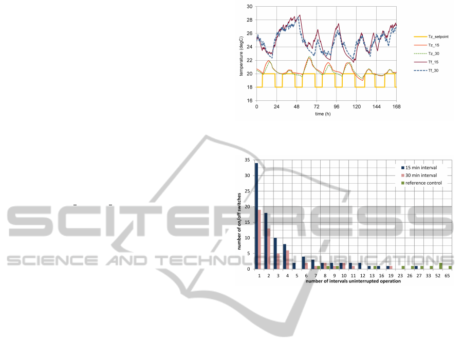
When the latter method is applied, the load duration

curves are similar to the results which are shown in

Figure 5. The interior temperatures have a minor dif-

ference, which is shown in Figure 9. In this Fig-

ure, the subscripts 15 and 30 indicate a 15 minute

and 30 minute time interval during simulation respec-

tively. The advantage of the 30 minute time interval

is shown in Figure 10, which shows the amount of

on/off switches in relation to the amount of uninter-

rupted running time intervals of the heat pump. For

the investigated week, the total amount of switches

reduces from 92 to 53. A further reduction can be ex-

pected when an additional charging constraint is in-

cluded for the domestic hot water storage, as most of

the heat pump switches are related to short charging

periods of this storage.

By comparison, the reference control switches

only 11 times. This is perhaps an advantage for the

service life of the heat pump, but Figure 6 demon-

strates drawbacks on the experienced comfort. The

on/off thermostats programmed for reference control

of the space heating and the domestic hot water stor-

age, cause too much cooling down of the house and

of the hot water storage, which results in long periods

of heating demand afterwards. This is observed from

the high number of intervals of uninterrupted opera-

tion of the heat pump in case of reference control in

Figure 10. For the reference control the longest pe-

riod is 65 time intervals of 15 minutes or 16.25 hours,

for the optimized control this is 19 time intervals of

30 minutes or 9.5 hours. In practice, a PID controller

to control the space heating demand would probably

perform better than the on/off reference control and

result in less cooling down of the house and more fre-

quent switching of the heat pumps. This should also

result in shorter operating times and possibly some re-

duction of the aggregated peak electrical loads com-

pared to the reference control.

Results for Periods with Less Heat Demand

As shown in Figure 5 and discussed on Section 5.1,

the peak electrical load is reduced signiﬁcantly for the

Figure 9: Temperature response for 15 and 30 minute time

intervals.

Figure 10: Amount of heat pump on/off switches related to

uninterrupted operation time intervals.

optimized control. It is interesting to verify if a simi-

lar result is found for periods with less heat demand.

In Figure 11, weather data of a different week for the

same location and climatic year is shown. The ag-

gregated electrical energy demand for the optimized

and reference control is shown in Figure 12. The in-

door temperatures (ﬂoor heating temperature Tf and

interior zone temperature Tz) for the same detached

house are shown in Figure 13.

During this week, the domestic hot water demand

dominates the aggregated electrical energy demand,

while the space heating demand is largely concen-

trated on one day between 72 and 96 hours. Due to

approximately 80% simultaneity in the operation of

the heat pumps for domestic hot water, the reference

control shows a high peak electrical demand of 145

kW. The optimized control reduces this to 45 kW.

Notice that the interior zone temperatures are ap-

proximately similar for the reference and optimized

control. The slightly increasing temperatures above

the setpoints which is seen on the last two days are

due to relatively high solar gains. The short term

up and down movement of the ﬂoor heating tempera-

tures from 0 up to 84 hours indicates frequent on/off

switching of the heat pump. Also in this case, the

heat pump switching is more frequent for the opti-

mized control than for the reference control. The total

SMARTGREENS2015-4thInternationalConferenceonSmartCitiesandGreenICTSystems

144

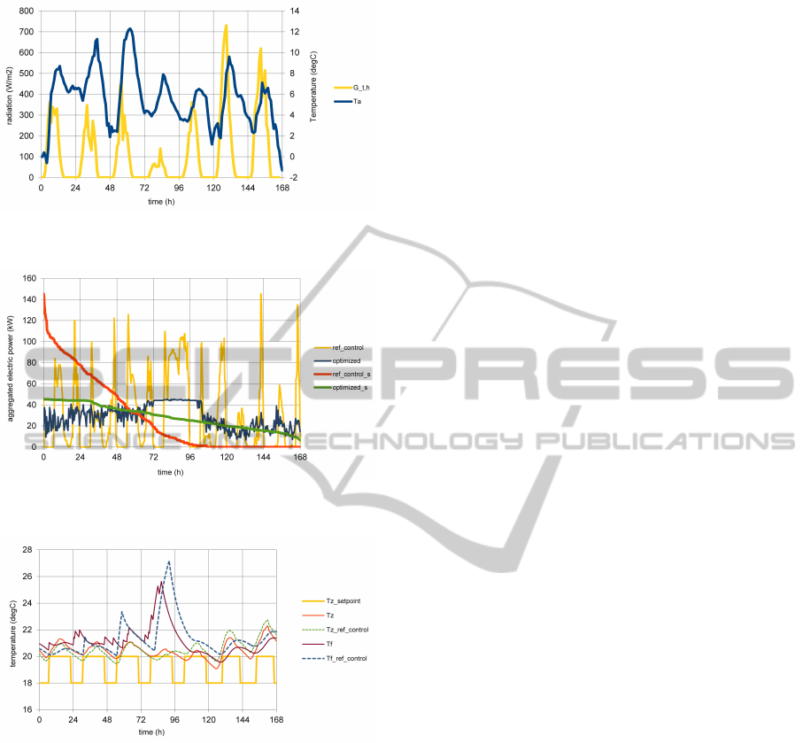
Figure 11: Input weather data for a week with less heat de-

mand.

Figure 12: Aggregated electrical energy demand for a week

with less heat demand.

Figure 13: Indoor temperatures for a week with less heat

demand.

amount of switches for this week is 32 for the opti-

mized control and 10 for the reference control. How-

ever, the longest period of uninterrupted heat pump

operation is 3 hours for the optimized control and

10.25 hours for the reference control, which increases

the chance for simultaneity and hence explains the

high peak electrical load of the reference control. This

also has a relation with the schedules shown in Figure

3. As young families and young couples dominate

the district’s population and the applied schedules for

domestic hot water demand and interior temperature

setpoints of these occupancy types are approximately

similar, the chance for simultaneity is high. A com-

monly used hot water storage contains a single tem-

perature sensor. Within the storage, a good degree of

temperature stratiﬁcation of hot and cold water layers

is present. In that case, a PID controller would not

perform much better than the simple on/off reference

control.

Optimality of the Control

The main objective for the optimization is to mini-

mize peak electricity consumption. Besides this ob-

jective, there are some hard constraints on the thermal

comfort, i.e. a minimum temperature, maximum size

of the ﬂexible space heating storage and minimum

hot water storage state of charge. Besides that, a 30

minute time interval is introduced during optimization

to avoid excessive on/off switching of the heat pumps.

Hence, the deﬁnition of what is in this case really ”op-

timum” for the control is not so obvious. As our re-

sults show, the peak electricity decreases signiﬁcantly

as the result of the optimized control, but there is a

trade off between the quality of this objective, reach-

ing comfort temperatures in the house which are close

to the setpoints and limiting the amount of heat pump

on/off switches.

6 CONCLUSIONS AND FUTURE

WORK

Optimal control on a central or aggregated level of a

group of heat pumps used for providing space heating

and domestic hot water is investigated. It is demon-

strated that model predictive control is required in

order to anticipate on changing weather conditions

and occupancy related thermal gains and losses. The

developed control algorithm is very well capable to

reach multiple objectives, i.e. minimize peak electri-

cal demands and maintain adequate thermal comfort

levels for each household in terms of comfortable, de-

sired operative temperatures and sufﬁcient charging

states of the buffers to supply domestic hot water.

For the simulation case which involves 104

houses, it takes 100 seconds to compute the heat

pump planning for 7 days in advance with 15 minute

time intervals, on a PC with Intel quad core processor

and 8 GB internal memory. Thus acceptable com-

putational effort for this type of control is demon-

strated. For larger district scales, the computational

time can be limited further by shorter planning hori-

zons, a larger time interval and applying the more ef-

ﬁcient time scale MILP algorithm.

A comparison with simulated results using a ref-

erence control algorithm which equals existing non-

optimized, individual heat pump control, demon-

strates for the optimized, central control, a substan-

tial decrease of the aggregated electricity demand

CentralModelPredictiveControlofaGroupofDomesticHeatPumps-CaseStudyforaSmallDistrict

145

peaks and improved thermal comfort for the residents.

However, the optimized control causes a signiﬁcant

increase of the amount of heat pump on/off switches,

which can be decreased by increasing the time period

of the optimization and by deﬁning additional con-

straints on charging the domestic hot water storage.

Future work is aimed at developing predictive

models for home space heating and domestic hot wa-

ter demand in which online learning is incorporated

and at studying cases which involve cooling during

the summer months. We will also apply the devel-

oped simulation environment to applications which

are more complex and require additional control al-

gorithms. Besides that, we will further compare

the quality of central control with individual control

where optimization is based on auction principles.

ACKNOWLEDGEMENT

The authors would like to thank the Dutch national

program TKI-Switch2SmartGrids for supporting the

project Meppelenergy and the STW organization for

supporting the project I-Care 11854.

REFERENCES

AgentschapNL (2013). Reference houses 2013 (in

dutch: Referentiewoningen nieuwbouw 2013).

http://www.rvo.nl/sites/default/ﬁles/2013/09/ Refer-

entiewoningen.pdf, visited October 2014.

Alpha-Innotec (2014). Alpha-Innotec instruction and

user manual WZS series brine/water heat pumps (in

Dutch).

Bakker, V. (2011). Triana: a control strategy for Smart

Grids: Forecasting, planning & real-time control.

PhD thesis, University of Twente.

Blokker, E. and Poortema, K. (2007). Effect study domestic

hot water (in dutch: Effecten levering warm tapwater

door derden). Technical report, KIWA.

Bosman, M. (2012). Planning in Smart Grids. PhD thesis,

University of Twente.

Claessen, F., Claessens, B., Hommelberg, M., Molderink,

A., Bakker, V., and Toersche, H. (2014). Comparative

analysis of tertiary control systems for smart grids us-

ing the ﬂex street model. Renewable energy, 69:260–

270.

Dar, U. I., Sartori, I., Georges, L., and Novakovic, V.

(2014). Advanced control of heat pumps for improved

ﬂexibility of net-zeb towards the grid. Energy and

Buildings, 69:74–84.

Dreijerink, L. and Uitzinger, J. (2013). Socio-economic

evaluation report apeldoorn. Technical report, IVAM

University of Amsterdam. EU SORCER project.

Dufﬁe, J. A. and Beckman, W. A. (1980). Solar engineering

of thermal processes. Wiley, New York.

ECN (2014). Energy trends 2014 (in dutch: En-

ergie trends 2014). Technical report, ECN.

http://energietrends.info/, visited December 2014.

Erbs, D. G., Klein, S. A., and Dufﬁe, J. A. (1982). Estima-

tion of the diffuse radiation fraction for hourly, daily

and monthly-average global radiation. Solar Energy,

28(4):293–302.

Fink, J. and Hurink, J. L. (2015). Minimizing costs is easier

than minimizing peaks when supplying the heat de-

mand of a group of houses. European journal of op-

erational research, 242(2):644–650.

Fink, J., Leeuwen, R. v., Hurink, J., and Smit, G. (2014).

Linear programming control of a group of heat pumps.

ESEIA 2014 conference, submitted to Journal Energy,

Sustainability and Society.

Halvgaard, R., Poulsen, N., Madsen, H., and Jorgensen, J.

(2012). Economic model predictive control for build-

ing climate control in a smart grid. Proceedings of

2012 IEEE PES innovative Smart Grid Technologies

(ISGT).

Hepbasli, A. and Kalinci, Y. (2009). A review of heat pump

water heating systems. Renewable and Sustainable

Energy Reviews, 13(6):1211–1229.

Janssen-Visschers, I. and Lee, G. v. d. (2013). Vision on

electricity sector production and tax development (in

dutch: Visie op productie- en belastingontwikkelingen

in de elektriciteitssector). Technical report, Tennet.

Kok, J., Warmer, C., and Kamphuis, I. (2005). Power-

matcher: multiagent control in the electricity infras-

tructure. In Proceedings of the fourth international

joint conference on Autonomous agents and multia-

gent systems, pages 75–82.

Leeuwen, R. v., Fink, J., Wit, J. d., and Smit, G. (2014).

Thermal storage in a heat pump heated living room

ﬂoor for urban district power balancing, effects on

thermal comfort, energy loss and costs for residents.

In Smartgreens 2014, Barcelona. INSTICC.

Leeuwen, R. v., Wit, J. d., Fink, J., and Smit, G. (2015).

Low-energy house thermal model parameter estima-

tion for smart grid control. submitted to conference

IEEE-Powertech 2015.

Madsen, H. and Holst, J. (1995). Estimation of continuous-

time models for the heat dynamics of a building. En-

ergy and Buildings(1995) 67-79.

Meppelenergie (ND). Meppel energy (in dutch: Meppel

energie). http://www.meppelenergie.nl/nieuwveense-

landen, visited March 2014.

Milieucentraal (ND). Insights into energy consump-

tion (in dutch: Inzicht in uw energiereken-

ing). http://www.milieucentraal.nl/, visited December

2014.

Mitchel, J. W. and Braun, J. E. (2013). Principles of Heat-

ing, Ventilation, and Air Conditioning in buildings.

Wiley, New York.

Molderink, A., Bakker, V., Bosman, M. G., Hurink, J. L.,

and Smit, G. J. (2010). A three-step methodology

to improve domestic energy efﬁciency. In Innova-

tive Smart Grid Technologies (ISGT), 2010, pages 1–

8. IEEE.

Oldewurtel, F., Parisio, A., Jones, C. N., Gyalistras, D., Gw-

erder, M., Stauch, V., Lehmann, B., and Morari, M.

SMARTGREENS2015-4thInternationalConferenceonSmartCitiesandGreenICTSystems

146

(2012). Use of model predictive control and weather

forecasts for energy efﬁcient building climate control.

Energy and Buildings, 45:15–27.

ıvara, S.,

Sirok

y, J., Ferkl, L., and Cigler, J. (2011).

Model predictive control of a building heating sys-

tem: The ﬁrst experience. Energy and Buildings,

43(2):564–572.

Scheepers, M., Seebregts, A., Hanschke, C., and Nieuwen-

hout, F. (2007). Inﬂuence of innovative technology on

the future electricity infrastructure (in dutch: Invloed

van innovatieve technologie op de toekomstige elek-

triciteitsinfrastructuur). Technical report, ECN.

Sirok

y, J., Oldewurtel, F., Cigler, J., and Pr

ıvara, S. (2011).

Experimental analysis of model predictive control for

an energy efﬁcient building heating system. Applied

Energy, 88(9):3079–3087.

TESS (ND). Trnsys transient system simulation tool.

http://www.trnsys.com/, visited December 2014.

CentralModelPredictiveControlofaGroupofDomesticHeatPumps-CaseStudyforaSmallDistrict

147