
A Many-objective Optimization Framework for Virtualized Datacenters
Fabio L
´
opez Pires
1,2
and Benjam
´
ın Bar
´
an
2,3
1
Itaipu Technological Park (PTI), Hernandarias, Paraguay
2
National University of Asunci
´
on (UNA), San Lorenzo, Paraguay
3
National University of the East (UNE), Ciudad del Este, Paraguay
Keywords:
Virtual Machine Placement, Many-objective Optimization, Datacenter, Virtualization, Cloud Computing.
Abstract:
The process of selecting which virtual machines should be located (i.e. executed) at each physical machine of
a datacenter is commonly known as Virtual Machine Placement (VMP). This work presents a general many-
objective optimization framework that is able to consider as many objective functions as needed when solving
the VMP problem in a pure multi-objective context. As an example of utilization of the proposed framework,
for the first time a formulation of the many-objective VMP problem (MaVMP) is proposed, considering the
simultaneous optimization of the following five objective functions: (1) power consumption, (2) network traf-
fic, (3) economical revenue, (4) quality of service and (5) network load balancing. To solve the formulated
many-objective VMP problem, an interactive memetic algorithm is proposed. Simulations prove the correct-
ness of the proposed algorithm and its effectiveness converging to a treatable number of solutions in different
experimental scenarios.
1 INTRODUCTION
One of the key challenges in modern datacenters is
to efficiently manage power consumption, conside-
ring electricity costs and the carbon dioxide foot-
prints (Beloglazov et al., 2011). Most of the time,
servers operate in a very low energy-efficiency re-
gion (i.e. between 10 and 50% of resource utiliza-
tion), even considering that workload peaks rarely
occur in practice (Barroso and H
¨
olzle, 2007). Conse-
quently, applying techniques for higher resource uti-
lization can result in more energy-efficient server ope-
ration. Virtualization of computational resources is a
technology that dynamically improves the utilization
of available resources in a datacenter according to the
existing demand, improving efficiency. Correctly lo-
cating virtual machines (VMs) into physical machines
(PMs) reduces the amount of hardware in use, let-
ting unused PMs to be in standby mode or even to
shut down. This way, average resource utilization as
well as energy efficiency may be improved, resulting
in better economical revenue and greener datacenters.
Virtualization in modern datacenters introduces
management decisions related to the placement of
VMs. In this context, Virtual Machine Placement
(VMP) is the process of selecting which VMs should
be executed in a given set of PMs of a datacenter.
1.1 Background and Motivation
In datacenters with a considerable amount of PMs
and VMs, there is a large number of possible criteria
that can be considered when selecting a placement,
depending on the priorities and optimization objec-
tives. These criteria can even change from one period
of time to another, which implies a variety of possi-
ble formulations of the VMP problem and objective
functions to be optimized for virtualized datacenters.
According to (L
´
opez Pires and Bar
´
an, 2015), the
optimization of the energy consumption is the most
studied objective function in VMP literature (Sun
et al., 2013; Beloglazov et al., 2012). On the other
hand, network traffic (Anand et al., 2013), economi-
cal revenue (Shi et al., 2013; Sato et al., 2013), per-
formance (Bin et al., 2011) and resource utilization
(Mishra and Sahoo, 2011) optimization are also very
studied. For each objective function, several possible
formulations can be proposed.
In the VMP context, objective functions can be
studied according to the following identified opti-
mization approaches: (1) mono-objective (MOP), (2)
multi-objective solved as mono-objective (MAM) and
(3) multi-objective (PMO) (L
´
opez Pires and Bar
´
an,
2015). The mono-objective approach considers the
optimization of only one objective or the individual
439
López Pires F. and Barán B..
A Many-objective Optimization Framework for Virtualized Datacenters.
DOI: 10.5220/0005434604390450
In Proceedings of the 5th International Conference on Cloud Computing and Services Science (CLOSER-2015), pages 439-450
ISBN: 978-989-758-104-5
Copyright
c
2015 SCITEPRESS (Science and Technology Publications, Lda.)

optimization of more than one objective, one at a
time. On the other hand, multi-objective solved as
mono-objective approach considers the optimization
of multiple objectives combined into one objective
(usually as a weighted sum of different normalized
objectives), while a pure multi-objective approach
considers the simultaneous optimization of different
(possible contradictory) objectives. To the best of
the authors’ knowledge, there is no many-objective
optimization formulation proposed for the VMP pro-
blem in the specialized literature (L
´
opez Pires and
Bar
´
an, 2015), i.e a multi-objective optimization pro-
blem with at least four conflicting objective functions
(von L
¨
ucken et al., 2014).
Considering the large number of existing objective
functions for the VMP problem, this work presents a
many-objective optimization framework to be able to
consider as many objective functions as needed when
solving the VMP problem. As an example of uti-
lization of the proposed framework, for the first time
a formulation of the many-objective VMP problem
(MaVMP) is proposed, considering the following five
objective functions: (1) power consumption minimi-
zation, (2) network traffic minimization, (3) economi-
cal revenue maximization, (4) QoS maximization and
(5) network load balancing optimization. In the pre-
sented formulation, a multi-level priority is associa-
ted to each VM, representing a Service Level Agree-
ment (SLA) considered in the placement process. To
solve the formulated MaVMP problem, an interactive
memetic algorithm is proposed considering the is-
sues that give place the formulated problem of many-
objective optimization for Pareto-based algorithms.
This paper is structured in the following way: Sec-
tion 2 presents a multi-objective optimization pro-
blem formulation, considering the issues that give
place the problem of many-objective optimization.
Section 3 details the proposed general many-objective
optimization framework, while Section 4 summarizes
a many-objective formulation of the VMP problem
considering the simultaneous optimization of five ob-
jective functions and a multi-level priority of SLA.
Section 5 presents a novel interactive memetic al-
gorithm proposed for solving the formulated many-
objective problem, while Section 6 presents first expe-
rimental results. Finally, conclusions and future work
are left to Section 7.
2 MULTI-OBJECTIVE
OPTIMIZATION
A general pure multi-objective optimization problem
(PMO) includes a set of p decision variables, q objec-
tive functions, and r constraints. Objective functions
and constraints are functions of decision variables. In
a PMO formulation, x represents the decision vector,
while y represents the objective vector. The decision
space is denoted by X and the objective space as Y .
These can be expressed as (Coello et al., 2007):
Optimize:
y = f (x) = [ f
1
(x), f
2
(x),..., f
q
(x)] (1)
subject to:
e(x) = [e
1
(x),e
2
(x),...,e
r
(x)] ≥ 0 (2)
where:
x = [x
1
,x
2
,...,x
p
] ∈ X (3)
y = [y
1
,y
2
,...,y
q
] ∈ Y (4)
It is important to remark that optimizing, in a parti-
cular problem context, can mean maximizing or mi-
nimizing. The set of constrains e(x) ≥ 0 defines the
set of feasible solutions X
f
⊂ X and its corresponding
set of feasible objective vectors Y
f
⊂ Y . The feasible
decision space X
f
is the set of all decision vectors x in
the decision space X that satisfies the constraints e(x),
and it is defined as:
X
f
= {x | x ∈ X ∧ e(x) ≥ 0} (5)
The feasible objective space Y
f
is the set of the ob-
jective vectors y that represents the image of X
f
onto
Y and it is denoted by:
Y
f
= {y | y = f (x) ∀x ∈ X
f
} (6)
To compare two solutions in a multi-objective
context, the concept of Pareto dominance is used.
Given two feasible solutions u, v ∈ X, u dominates v,
denoted as u v, if f (u) is better or equal to f (v) in
every objective function and strictly better in at least
one objective function. If neither u dominates v, nor
v dominates u, u and v are said to be non-comparable
(denoted as u ∼ v).
A decision vector x is non-dominated with respect
to a set U, if there is no member of U that dominates x.
The set of non-dominated solutions of the whole set of
feasible solutions X
f
, is known as optimal Pareto set
P
∗
. The corresponding set of objective vectors consti-
tutes the optimal Pareto front PF
∗
.
PMOs with more than three objective functions
are known as Many-Objective Optimization Problems
(MaOPs), as defined in (Cheng et al., 2014). MaOPs
differ significantly from PMOs because several issues
should be considered when solving problems with
more than three objective functions (Farina and Am-
ato, 2002). In case of Pareto-based algorithms, these
CLOSER2015-5thInternationalConferenceonCloudComputingandServicesScience
440

issues are intrinsically related to the fact that as the
number of objective increases, the proportion of non-
dominated elements in the population grows, being
increasingly difficult to discriminate among solutions
using only the Pareto dominance relation (Deb et al.,
2006). Additionally, determining which solution to
keep and which to discard in order to converge toward
the Pareto set is still a relevant issue to be addressed
(Farina and Amato, 2002). Pareto-based algorithms
are still not able to provide the required selection pres-
sure towards better solutions in order to conduct an
efficient evolutionary search and, even elitism may be
difficult. As the number of objectives grows, the pro-
portion of non-comparable solutions to the total num-
ber of solutions tends to one (von L
¨
ucken et al., 2014),
making more difficult to solve a MaOP. Clearly, diffi-
culties in solving MaOPs explain why it has not yet
been studied in the VMP literature.
3 MANY-OBJECTIVE
OPTIMIZATION FRAMEWORK
The general many-objective optimization framework
for the VMP problem proposed in this work consi-
ders that as the number of conflicting objectives of
a MaVMP problem formulation increases, the total
number of non-dominated solutions increases (even
exponentially in some cases), being increasingly dif-
ficult to discriminate among solutions using only the
dominance relation (Farina and Amato, 2002). For
this reason, this work proposes the utilization of lower
and upper bounds associated to each objective func-
tion z ∈ {1,...,q} (L
z
≤ f
z
(x) ≤ U
z
) to be able to
reduce iteratively the number of possible compro-
mise solutions of the Pareto set approximation, when
needed by the decision maker.
A VMP formulation, based on many objective
functions and constraints to be detailed in Section 4,
may be written as:
Optimize:
y = f (x) = [ f
1
(x), f
2
(x),..., f
q
(x)] (7)
where:
f
1
(x) = power consumption minimization
f
2
(x) = network traffic minimization
f
3
(x) = economical revenue maximization
f
4
(x) = QoS maximization
f
5
(x) = network load balancing optimization
.
.
.
f
q
(x) = any other considered function
(8)
subject to:
e
1
(x) : unique placement of VMs;
e
2
(x) : assure provisioning of highest SLA;
e
3
(x) : processing resource capacity of PMs;
e
4
(x) : memory resource capacity of PMs;
e
5
(x) : storage resource capacity of PMs;
e
6
(x) : f
1
(x) ∈ [L
1
,U
1
];
e
7
(x) : f
2
(x) ∈ [L
2
,U
2
];
e
8
(x) : f
3
(x) ∈ [L
3
,U
3
];
e
9
(x) : f
4
(x) ∈ [L
4
,U
4
];
e
10
(x) : f
5
(x) ∈ [L
5
,U
5
];
.
.
.
e
r
(x) : any other considered constraint.
(9)
4 MANY-OBJECTIVE VIRTUAL
MACHINE PLACEMENT
A few articles proposed formulations of a pure
multi-objective VMP problem (MVMP) (Gao et al.,
2013; L
´
opez Pires and Bar
´
an, 2013), considering the
simultaneous optimization of at most three objective
functions. To the best of the authors’ knowledge,
this work proposes for the first time the formulation
of a MaVMP problem considering the following five
objective functions to be simultaneously optimized:
(1) power consumption, (2) network traffic, (3)
economical revenue, (4) quality of service and (5)
network load balancing. In this many-objective for-
mulation, a multi-level priority is associated to each
VM, representing a SLA. Formally, the proposed
offline many-objective optimization VMP problem
can be enunciated as:
Given a set of PMs, H = {H
1
,H
2
,...,H
n
}, a
network topology G (as illustrated in Figure 1) and a
set of VMs, V = {V
1
,V
2
,...,V
m
}, it is sought a correct
placement of the set of VMs V in the set of PMs
H satisfying the r constraints of the problem and
simultaneously optimizing all q objective functions
defined in this formulation (as energy consumption,
network traffic, economical revenue, QoS and load
balancing in the network), in a pure many-objective
context.
4.1 Input Data
The proposed formulation of the VMP problem mo-
dels a virtualized datacenter infrastructure, composed
by PMs and a network topology. The set of PMs
AMany-objectiveOptimizationFrameworkforVirtualizedDatacenters
441

is represented as a matrix H of dimension (n x 4).
Each H
i
is represented by processing resources CPU
(as ECU)
1
, RAM memory [GB], storage [GB] and a
maximum power consumption [W] as:
H
i
= [Hcpu
i
,Hram
i
,Hhdd
i
, pmax
i
]
∀i ∈ {1,...,n}
(10)
where:
Hcpu
i
: Processing resources of H
i
;
Hram
i
: Memory resources of H
i
;
Hhdd
i
: Storage resources of H
i
;
pmax
i
: Maximum power consumption of H
i
;
n: Number of PMs.
As shown in Figure 1, the network topology of
the virtualized datacenter is represented as:
G: Network topology;
L: Set of links l
a
in G. For simplicity, we
assume that all links are semi-duplex;
M: Set of paths for all-to-all PM interconnec-
tions;
K: Capacity set of the communication cha-
nnel, typically in [Mbps].
The set of VMs requested by customers is repre-
sented as a matrix V of dimension (m x 5). Each V
j
requires processing resources CPU (as ECU)
1
, RAM
memory [GB] and storage [GB], providing for them
an economical revenue R
j
[$] for the provider. A SLA
is also assigned to each VM to indicate its level of
priority. Consequently, a V
j
is represented as:
V
j
= [V cpu
j
,V ram
j
,V hdd
j
,R
j
,SLA
j
]
∀ j ∈ {1,...,m}
(11)
where:
V cpu
j
: Processing requirements of V
j
;
V ram
j
: Memory requirements of V
j
;
V hdd
j
: Storage requirements of V
j
;
R
j
: Economical revenue for locating V
j
;
SLA
j
: Service Level Agreement SLA
j
of a V
j
. If
the highest priority level is s, then SLA
j
∈
{1,. . . , s};
m: Number of VMs.
The traffic between VMs is represented as a ma-
trix T of dimension (m x m). Each V
j
requires net-
work communication resources [Mbps] to communi-
cate with other VMs. These communication resources
1
http://aws.amazon.com/ec2/faqs
are represented as:
T
j
= [T
j1
,T
j2
,..., T
jm
]
∀ j ∈ {1,...,m}
(12)
where:
T
jk
: Average network traffic between V
j
and
V
k
[Mbps]. Note that we can consider
T
j j
= 0.
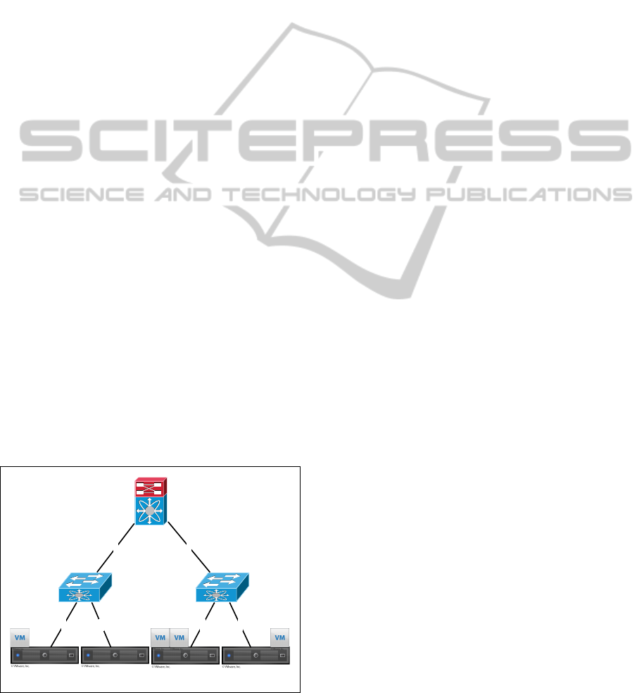
Figure 1 presents a basic example of a virtualized
datacenter infrastructure, composed by 4 PMs H =
{H
1
,H
2
,H
3
,H
4
} and a network topology considering
6 physical network links L = {l
1
,l
2
,l
3
,l
4
,l
5
,l
6
}. In
this example, the set of capacity for each communica-
tion channel is K = {100,100,100,100,1000, 1000}
[Mbps] respectively. Using shortest path, a path m
12
between H
1
and H
2
uses links {l
1
,l
2
}, i.e. m
12
=
{l
1
,l
2
}. Analogously, m
13
= {l
1
,l
5
,l
6
,l
3
} and m
14
=
{l
1
,l
5
,l
6
,l
4
}, as shown in Figure 1.
4.2 Output Data
A calculated solution should indicate the exact place-
ment of each VM V
j
on the necessary PMs H
i
,
considering the many-objective optimization criteria
applied. A placement (or possible solution to the
formulated problem) is represented in what follows
as a matrix P = {P
ji
} of dimension (m x n), where
P
ji
∈ {0,1} indicates if V
j
is located (P
ji
= 1) or not
(P
ji
= 0) for execution on a PM H
i
(i.e., P
ji
: V
j
→ H
i
).
4.3 Constraints
4.3.1 Constraint 1: Unique Placement of VMs
A VM V
j
should be located to run on a single PM H
i
or alternatively, it could be not located in any PM if
the associated SLA
j
is not the highest level of priority
s. Consequently, this constraint is expressed as:
n
∑
i=1
P
ji
≤ 1 ∀ j ∈ {1,...,m}
(13)
where:
P
ji
: Binary variable equals 1 if V
j
is located to
run on H
i
; otherwise, it is 0.
4.3.2 Constraint 2: Assure SLA Provisioning
A VM V
j
with the highest level of SLA (i.e. SLA
j
= s)
must necessarily be located to run on a PM H
i
. Con-
sequently, this constraint is expressed as:
n
∑
i=1
P
ji
= 1 ∀ j such that SLA
j
= s
(14)
CLOSER2015-5thInternationalConferenceonCloudComputingandServicesScience
442
4.3.3 Constraints 3-5: Physical Resource
Capacity of PMs
A PM H
i
must have sufficient available resources
to meet the requirements of all VMs V
j
that are lo-
cated to run on H
i
. In this work, it is not considered
the overbooking of resources (Tom
´
as and Tordsson,
2013). Consequently, this set of constraints can be
mathematically formulated as:
m
∑
j=1
V cpu
j
× P
ji
≤ Hcpu
i
(15)
m
∑
j=1
V ram
j
× P
ji
≤ Hram
i
(16)
m
∑
j=1
V hdd
j
× P
ji
≤ Hhdd
i
(17)
∀i ∈ {1,...,n},i.e. for all physical machine H
i
.
4.3.4 Adjustable Constraints
This work proposes the utilization of lower and upper
bounds associated to each objective function to re-
duce the number of possible solutions of the Pareto set
approximation P
known
, when needed by the decision
maker. Consequently, this set of adjustable bounds
can be mathematically formulated as the following
constraints:
f
z
(x) ∈ [L
z
,U
z
] ∀z ∈ {1,...,q}
(18)
4.4 Objective Functions
A VMP problem can be defined as a many-objective
optimization problem, considering the simultaneous
optimization of more than three objective functions.
l
5
l
6
H
1
H
2
H
3
H
4
l
1
l
2
l
3
l
4
Active paths of M
m
13
= {l
1,
l
5,
l
6,
l
3
}
m
14
= {l
1,
l
5,
l
6,
l
4
}
m
34
= {l
3,
l
4
}
V
3
V
1
V
2
100 Mbps 100 Mbps 100 Mbps 100 Mbps
1000 Mbps 1000 Mbps
V
4
Total traffic per path
m
13
= 4 Mbps
m
14
= 2 Mbps
m
34
= 4 Mbps
Figure 1: Example of placement in a virtualized datacenter
infrastructure, composed by PMs and a network topology.
As a concrete example, this work proposes for the first
time the optimization of the following five objective
functions:
4.4.1 Power Consumption Minimization
Based on (Beloglazov et al., 2012) formulation, this
work also proposes the minimization of power con-
sumption, represented by the sum of the power con-
sumption of each PM H
i
:
f
1
(x) =
n
∑
i=1
((pmax
i
− pmin
i
) ×Ucpu
i
+ pmin
i
) ×Y
i
(19)
where:
f
1
(x): Total power consumption of the PMs;
pmin
i
: Minimum power consumption of H
i
. In
what follows, pmin
i
= pmax
i
∗ 0.6 (Belo-
glazov et al., 2012);
Ucpu
i
: Utilization ratio of processing resources
used by H
i
;
Y
i
: Binary variable equals 1 if H
i
is turned
on; otherwise, it is 0.
4.4.2 Network Traffic Minimization
(Shrivastava et al., 2011) proposed the minimization
of network traffic among VMs by maximizing local-
ity. Based on this approach, this work proposes equa-
tion (20) to estimate network traffic represented by the
sum of average network traffic generated by each VM
V
j
, that is located to run on any PM, with other VMs
V
k
that are located to run on different PMs.
f
2
(x) =
m
∑
j=1
m
∑
k=1
(T
jk
× D
jk
) (20)
where:
f
2
(x): Total network traffic among VMs;
D
jk
: Binary variable that equals 1 if V
j
and V
k
are located in different PMs; otherwise, it
is 0.
The traffic between two VMs V
j
and V
k
which are
located on the same PM H
i
do not contribute to in-
crease the total network traffic given by equation (20);
therefore, D
jk
= 0 if P
ji
= P
ki
= 1.
4.4.3 Economical Revenue Minimization
Based on (L
´
opez Pires and Bar
´
an, 2013), this work
presents equation (21) to estimate the total economi-
cal revenue that a datacenter receives for meeting the
requirements of its customers, represented by the sum
AMany-objectiveOptimizationFrameworkforVirtualizedDatacenters
443

of the economical revenue obtainable by each VM V
j
placement that is effectively located for execution on
any PM.
f
3
(x) =
m
∑
j=1
(R
j
× X
j
) (21)
where:
f
3
(x): Total economical revenue for placing
VMs;
X
j
: Binary variable that equals 1 if V
j
is lo-
cated for execution on any PM; other-
wise, it is 0.
4.4.4 QoS Maximization
In this work, the QoS maximization proposes to lo-
cate the maximum number of VMs with the highest
level of priority associated to the SLA. This objective
function is proposed in equation (22).
f
4
(x) =
m
∑
j=1
(
ˆ
C
SLA
j
× SLA
j
× X
j
) (22)
where:
f
4
(x): Total QoS figure for a given placement;
ˆ
C: Constant, large enough to prioritize ser-
vices with larger SLA over the ones with
lower SLA (see example in Section 4.4.6).
4.4.5 Network Load Balancing Optimization
This work calculates the total amount of traffic going
through a semi-duplex link l
a
as:
T
l
a
=
n
∑
i=1
n
∑
i
0
=1
F
aii
0
×
m
∑
j=1
m
∑
j
0
=1
P
ji
× P
j
0
i
0
× D
j j
0
× T
j j
0
!
(23)
where:
T l
a
: Total amount of traffic going through link
l
a
[Mbps];
F
aii
0
: Binary variable that equals 1 if l
a
∈ m
ii
0
;
otherwise, it is 0.
Inspired in (Donoso et al., 2005) formulation,
this work calculates the Maximum Link Utilization
(MLU) as:
MLU = max
∀l
a
∈L
T l
a
Cl
a
(24)
where:
MLU: Maximum Link Utilization;
Cl
a
: Channel capacity of link l
a
[Mbps].
In this paper, the load balancing optimization of
the network is formulated as the minimization of the
MLU, i.e.,
f
5
(x) = MLU (25)
4.4.6 Example
The following example details how the values of f
4
(x)
and f
5
(x) are calculated, considering the datacenter
infrastructure presented in Figure 1. For the other
three objective functions, see (L
´
opez Pires and Bar
´
an,
2013).
Consider the following placement matrix P where,
VMs V
1
and V
2
are executed in H
3
, while V
3
is exe-
cuted in H
1
and V
4
in H
4
:
P =
0 0 1 0
0 0 1 0
1 0 0 0
0 0 0 1
(26)
Additionally, consider
ˆ
C = 100 and the values of SLA
j
and X
j
presented in Table 1, f
4
(x) is calculated as:
f
4
(x) =
ˆ
C
SLA
1
× SLA
1
× X
1
+ ··· +
ˆ
C
SLA
4
× SLA
4
× X
4
= 100
2
× 2 × 1 + ··· + 100
3
× 3 × 1
= 3.06X10
6
(27)
It is important to remark that if
ˆ
C is not sufficiently
large, f
4
(x) could prefer a large number of VMs with
lower priority. As an example, if
ˆ
C = 1, 2 VMs with
SLA
j
= 2 result in a better figure of f
4
(x) than 1 VM
with SLA
j
= 3, what is not correct according to what
was presented in Section 4.4.4.
On the other hand, considering that each VM V
j
communicates at 1 [Mbps] with any other V
k
(k 6= j),
the placement P results in the values of T l
a
and Cl
a
presented in Table 2. So f
5
(x) is calculated as:
f
5
(x) = max
T l
1
Cl
1
,
T l
2
Cl
2
,
T l
3
Cl
3
,
T l
4
Cl
4
,
T l
5
Cl
5
,
T l
6
Cl
6
= max
6
100
,
0
100
,
8
100
,
6
100
,
6
1000
,
6
1000
=
8
100
(28)
5 INTERACTIVE MEMETIC
ALGORITHM
A Memetic Algorithm (MA) could be understood as
an Evolutionary Algorithm (EA) that in addition to
CLOSER2015-5thInternationalConferenceonCloudComputingandServicesScience
444

Table 1: Data for requested VMs used in basic example (see
Section 4.4.6).
V
j
SLA
j
X
j
V
1
2 1
V
2
2 1
V
3
2 1
V
4
3 1
Table 2: Data of network links used in basic example (see
Section 4.4.6).
l
a
T l
a
[Mbps] Cl
a
[Mbps] T l
a
/Cl
a
l
1
6 100 6/100
l
2
0 100 0/100
l
3
8 100 8/100
l
4
6 100 6/100
l
5
6 1000 6/1000
l
6
6 1000 6/1000
MLU 8/100
the standard selection, crossover and mutation opera-
tors of most Genetic Algorithms (GA) includes a local
optimization operator to obtain good solutions even at
early generations of an EA (B
´
aez et al., 2007).
This work proposes an interactive memetic al-
gorithm for solving the VMP problem in a many-
objective context, considering the proposed formu-
lation presented in Section 4 to simultaneously opti-
mize the five objective functions presented in the pre-
vious section. The proposed algorithm is extensible to
consider as many objective functions as needed while
only minor modifications may be needed if the num-
ber of objective functions changes.
It was shown in (von L
¨
ucken et al., 2014) that
many-objective optimization using Multi-Objective
Evolutionary Algorithms (MOEAs) is an active re-
search area, having multiple challenges that need to
be addressed regarding scalability analysis, visualiza-
tion of the results, algorithm design and experimen-
tal algorithm evaluation. The interactive memetic al-
gorithm presented in this section as a viable way to
solve a many-objective VMP problem, proposes the
inclusion of desirable ranges of values for the objec-
tive functions costs in order to interactively control
the possible huge number of feasible non-dominated
solution, as described in Section 2. The proposed in-
teractive memetic algorithm is based on the one pro-
posed in (L
´
opez Pires and Bar
´
an, 2013) and works as
follows:
In step 1, it is verified if the problem has at least
one solution (considering only VMs with SLA
j
= s)
to continue with next steps. If there is no possible so-
lution to the problem, the algorithm returns an appro-
priate error message. If the problem has at least one
solution, the algorithm proceeds to step 2, which ge-
nerates a set of random candidates P
0
, whose solu-
tions are repaired at step 3 to ensure that P
0
con-
tains only feasible solutions. Then, the algorithm tries
to improve candidates at step 4 using local search.
With the obtained non-dominated solutions, the first
set P
known
(Pareto set approximation) is generated at
step 5. After initialization in step 6, evolution begins
(iterations between steps 7 and 18).
The evolutionary process basically follows the
same behavior: solutions are selected from the union
of P
known
with the evoluationary set of solutions (or
population) also known as P
t
(step 8), crossover and
mutation operators are applied as usual (step 9), and
eventually solutions are repaired, as there may be in-
feasible solutions (step 10). Improvements of solu-
tions of the evolutionary population P
t
may be gen-
erated at step 11 using local search (local optimiza-
tion operators). At step 12, the Pareto set approxi-
mation P
known
is updated (if applicable); while at step
13 the generation (or iteration) counter is updated. At
step 15 the decision maker adjust the lower and upper
bounds if it is necessary, while at step 17 a new evo-
lutionary population P
t
is selected. The evolutionary
process is repeated until the algorithm meets a stop-
ping criterion (such as a maximum number of gen-
erations), finally returning the set of non-dominated
solutions P
known
in step 19.
Algorithm 1: Interactive Memetic Algorithm.
Data: datacenter infrastructure (see Section 4.1)
Result: Pareto set approximation P
known
1 check if the problem has a solution
2 initialize set of solutions P
0
3 P
0
0
= repair infeasible solutions of P
0
4 P
00
0
= apply local search to solutions of P
0
0
5 update set of solutions P
known
from P
00
0
6 t = 0; P
t
= P
00
0
7 while is not stopping criterion do
8 Q
t
= selection of solutions from P
t
∪ P
known
9 Q
0
t
= crossover and mutation of solutions of Q
t
10 Q
00
t
= repair infeasible solutions of Q
0
t
11 Q
000
t
= apply local search to solutions of Q
00
t
12 update set of solutions P
known
from Q
000
t
13 increment t
14 if interaction is needed then
15 ask for decision maker action (L
z
and U
z
)
16 end
17 P
t
= non-dominated sorting from P
t
∪ Q
000
t
18 end
19 return Pareto set approximation P
known
5.1 Population Initialization
Initially, a set of solutions (or population P
0
) is ran-
donmly generated. Each solution (or individual) is
represented as C = [C
1
,C
2
,. . . ,C
m
]. The possible val-
AMany-objectiveOptimizationFrameworkforVirtualizedDatacenters
445

ues that can take each C
k
for VMs with the highest
value of SLA
j
(SLA
j
= s) are in the range [1, n]. For
VMs V
j
with SLA
j
< s, the possible values are in the
range [0, n]. Within these ranges defined by the SLA
j
of each V
j
, the algorithm ensures at the initialization
stage that all VMs V
j
with the highest level of prio-
rity will be located for execution on a PM H
i
, while
for VMs V
j
with lower levels of priority SLA
j
, there
is always a probability larger than 0 that they may not
be located for execution in any PM.
5.2 Infeasible Solution Reparation
With a random generation at the initialization phase
(step 2 of Algorithm 1) and/or solutions generated by
standard genetic operators (step 9 of Algorithm 1), in-
feasible solutions may appear, i.e. the resources re-
quired by the VMs located for execution on certain
PMs could exceed the available resources (see Section
4.3.3), or one or more objectives functions may not
meet the adjustable constraints (see Section 4.3.4).
Repairing these infeasible solutions (steps 3 and
10 of Algorithm 1) may be done in two stages: first,
in the feasibility verification process, the population is
classified in two classes: feasible and infeasible (Al-
gorithm 2). Later, in the process of repairing infea-
sible solutions (Algorithm 3), the solutions which do
not meet the feasibility criteria are repaired in three
ways: (1) migrating some VMs to an available hard-
ware, (2) turning on some PMs and then migrating
VMs to them, or (3) turning off some VMs. Note that
at step 3 of Algorithm 3, V
j
migration to H
0
i
can be
done to other PMs, even if they are shut down.
Algorithm 2: Feasibility Verification
Data: set of solutions P
t
Result: set of feasible solutions P
0
t
1 while there are solutions not verified do
2 feasible = true ; i = 1
3 while i ≤ n and feasible = true do
4 if solution does not satisfy constraints (3-5)
then
5 feasible = false ; break
6 else
7 increment i
8 end
9 end
10 if feasible = false then
11 call Algorithm 3 (repair solution)
12 end
13 end
14 return set of feasible solutions P
0
t
Algorithm 3: Infeasible Solutions Reparation.
Data: infeasible solution
Result: feasible solution
1 feasible = false ; j = 1
2 while j ≤ m and feasible = false do
3 if it is possible then
4 migrate V
j
to H
0
i
(i
0
6= i)
5 else
6 if SLA
j
6= s then
7 turn off V
j
on H
i
8 else
9 replace solution with another solution
from P
known
10 end
11 end
12 end
13 return feasible solution
5.3 Local Search
Once a population contains only feasible solutions, a
local search is performed (steps 4 and 11 of Algorithm
1) for improving the solutions found so far in the evo-
lutionary population P
t
. The local search pseudo-code
is presented in Algorithm 4.
Algorithm 4: Local Search.
Data: set of feasible solutions P
0
t
Result: set of feasible optimized solutions P
00
t
1 probability = random number between 0 and 1
2 while there are solutions not verified do
3 if probability < 0.5 then
4 Try to turn off all the possible H
i
by
migrating all the V
j
assigned to H
0
i
with
available resources (i
0
6= i) and then try to
turn on all the possible V
j
(using SLA
j
priority order) assigning them to a H
i
with
available resources
5 else
6 Try to turn on all the possible V
j
(using
SLA
j
priority order) assigning them to a H
i
with available resources and then try to turn
off all the possible H
i
by migrating all the V
j
assigned to H
0
i
with available resources
(i
0
6= i)
7 end
8 end
9 return set of feasible optimized solutions P
00
t
For each individual in the population P
t
, the pro-
posed algorithm attempts to optimize a solution with a
local search (step 2 of Algorithm 4). For this purpose,
with probability
1
2
, the algorithm tries to maximize
the number of located VMs with higher level of prio-
rity, locating all possible VMs that were not located
so far, directly increasing f
4
(x) (total QoS) and f
3
(x)
(total economical revenue) (steps 3 to 5 of Algorithm
CLOSER2015-5thInternationalConferenceonCloudComputingandServicesScience
446

4). On the other hand, also with probability
1
2
, the al-
gorithm tries to minimize the number of PMs turned
on, directly reducing f
1
(x) (total power consumption)
(steps 6 to 8 of Algorithm 4). With the proposed prob-
abilistic local search method, a balanced exploitation
of objective functions (QoS, economical revenue and
power consumption) is achieved, as experimentally
verified with results presented in next section.
5.4 Fitness Function
The fitness function used in the proposed algorithm
is the one presented in (Deb et al., 2002). This fit-
ness value defines a non-domination rank in which
a value equal to its Pareto dominance level (1 is the
highest level of dominance, 2 is the next, and so on)
is assigned to each individual of the population. Bet-
ween two individuals with different non-domination
rank, the individual with lower value (higher level of
dominance) is considered better. To compare indivi-
duals with the same non-domination rank, a crowding
distance is used. The basic idea is to find the Eu-
clidean distance (properly normalized when the ob-
jectives have different measure units) between each
pair of individuals, based on the q objectives, in a
hyper-dimensional space (Deb et al., 2002). The in-
dividual with larger crowding distance is considered
better.
5.5 Variation Operators
The proposed interactive memetic algorithm uses a
Binary Tournament approach for selecting individuals
for crossover and mutation (Coello et al., 2007). The
crossover operator used in the presented work is the
single point cross-cut (Coello et al., 2007). The se-
lected individuals in the ascending population are re-
placed by descendants individuals.
This work uses a mutation method in which each
gene is mutated with a probability
1
m
, where m rep-
resents the number of VMs. This method offers the
possibility of full uniform gene mutation, with a very
low probability (but larger than zero), which is bene-
ficial to the exploration of the search space, reducing
the probability of stagnation in a local optimum.
The population evolution in the proposed inter-
active memetic algorithm is based on the population
evolution proposed in (Deb et al., 2002). A population
P
t+1
is formed from the union of the best known pop-
ulation P
t
and offspring population Q
t
, applying non-
domination rank and crowding distance operators.
5.6 Many-objective Considerations
Given that the number of non-dominated solutions
may rapidly increase, an interactive approach is re-
commended. That way, a decision maker can intro-
duce new constraints or adjust existing ones, while
the execution continues learning about the shape of
the Pareto front in the process. For simplicity, the
present work considers lower and upper bounds asso-
ciated to each objective function in order to help the
decision maker to reduce interactively the huge num-
ber of potencial solutions in the Pareto set approxi-
mation P
known
, while observing the evolution of its
corresponding Pareto front PF
known
.
6 EXPERIMENTAL RESULTS
To validate the proper operation of the proposed in-
teractive memetic algorithm for solving the MaVMP
on a purely many-objective context, different exper-
iments were proposed for problem instances consi-
dering both homogeneous as well as heterogeneous
hardware configurations of PMs, considering VMs
instance types offered by Amazon Elastic Compute
Cloud (EC2)
2
. Experiment 1 considered 2 problem
instances with homogeneous hardware configurations
of PMs (Hcpu = 4 [ECU], Hram = 16 [GB], Hhdd =
150 [GB], pmax = 1740 [W]), while Experiment 2
considered heterogeneous hardware configurations of
PMs according to Table 6.
A detailed description of the hardware of the VMs
instance types considered for the experiments is pre-
sented in Table 3. A general description of the con-
sidered problem instances is presented in Table 4,
while the complete set of datacenter infrastructure in-
put files used for the experiments with the correspon-
ding experimental results are available online
3
.
6.1 Experiment 1: Quality of Solutions
To compare the results obtained by the proposed in-
teractive memetic algorithm and to validate its proper
operation, an exhaustive search algorithm was also
implemented for finding all (n + 1)
m
possible solu-
tions of a given instance of the VMP problem, when
this alternative is computationally possible for the au-
thors. These results were compared to the results ob-
tained by the proposed interactive memetic algorithm
after evolving populations with 100 individuals for
100 generations. Both algorithms were implemented
2
http://aws.amazon.com/ec2/instance-types
3
https://sites.google.com/site/flopezpires/
AMany-objectiveOptimizationFrameworkforVirtualizedDatacenters
447

Table 3: Instance types of VMs considered in experiments.
For notation see equation (11).
Instance Type Vcpu Vram Vhdd R
t2.micro 1 1 0 9
t2.small 1 2 0 18
t2.medium 2 4 0 37
m3.medium 1 4 4 50
m3.large 2 8 32 100
m3.xlarge 4 15 80 201
m3.2xlarge 8 30 160 403
c3.large 2 4 32 75
c3.xlarge 4 8 80 151
c3.2xlarge 8 15 160 302
c3.4xlarge 16 30 320 604
c3.8xlarge 32 60 640 1209
r3.large 2 15 32 126
r3.xlarge 4 30 80 252
r3.2xlarge 8 61 160 504
r3.4xlarge 16 122 0 320
r3.8xlarge 32 244 0 320
Table 4: Problem instances considered in experiments, all
with 50% of VMs with the highest SLA s = 2.
Input File # PMs # VMs (n + 1)
m
3x5.vmp 3 5 1024
4x8.vmp 4 8 390625
12x50.vmp 12 50 ∼ 5X10
55
using ANSI C programming language (gcc)
4
and the
source code is also available online
3
.
Considering that this particular experiment aims
to validate the good level of exploration in the set of
feasible solutions X
f
, the local search of the algorithm
was disabled, strengthening its capability of explo-
ration rather than the rapid convergence to good so-
lutions even in early generations of the population.
For each problem instance considered in this ex-
periment (3x5.vmp and 4x12.vmp), one run of the ex-
haustive search algorithm was completed, obtaining
the optimal Pareto front PF∗ and its corresponding
Pareto set P∗. Furthermore, ten runs of the proposed
algorithm were completed, after evolving populations
of 100 individuals for 100 generations at each run.
The results obtained by the proposed algorithm for
each run were combined to obtain the Pareto front
PF
known
and its corresponding Pareto set P
known
. For
the 3x5.vmp and 4x8.vmp problem instances, the pro-
posed algorithm obtained every solution of the opti-
mal Pareto set and its corresponding Pareto front. A
summary of the number of elements in the correspon-
ding Pareto sets obtained are presented in Table 5.
4
http://gcc.gnu.org
Table 5: Summary of results obtained in Experiment 1 using
the proposed memetic algorithm (see Section 5).
Input File Name # P
∗
# P
known
% Found
3x5.vmp 51 51 100%
4x8.vmp 30 30 100%
Table 6: Types of PMs considered in Experiment 2. For
notation see equation (10).
PM Type Hcpu Hram Hhdd pmax
h1.medium 180 512 10000 1000
h1.large 350 1024 10000 1300
6.2 Experiment 2: Interactive Bounds
As mentioned in Section 3, this work proposes the
utilization of lower and upper bounds for each ob-
jective function f (z) (L
z
≤ f
z
(x) ≤ U
z
) to be able to
reduce iteratively the number of possible solutions of
the Pareto set approximation P
known
, when needed.
For the problem instance considered in this experi-
ment (12x50.vmp), one run of the proposed algorithm
was completed, after evolving populations of 100 in-
dividuals for 300 generations. The number of gener-
ations was incremented for this experiment from 100
to 300 considering the large number of possible solu-
tions for the particular problem considered (see Table
4). An interactive adjustment of the lower or upper
bounds associated to each objective function was per-
formed after every 100 generations in order to con-
verge to a treatable number of solutions.
It is important to remark that the interactive ad-
justment used in this experiment is only one of seve-
ral possible ones. As an example, we may consider:
(1) automatically adjusting 10% of the lower bounds
associated to maximization objective functions when
the Pareto front has more than 200 elements or (2)
manually adjusting upper bounds associated to mi-
nimization objective functions until the Pareto front
does not have more than 20 elements, just to cite a
pair of alternatives.
The Pareto front approximation PF
known
repre-
sents the complete set of Pareto solutions considering
unrestricted bounds (L
z
= −∞ and U
z
= ∞). On the
other hand, Pareto front approximation PF
reduced
rep-
resents the reduced set of Pareto solutions obtained by
interactively adjusting bounds L
z
and U
z
.
In the first 100 generations, the proposed al-
gorithm obtained 251 solutions with unrestricted
bounds. A decision maker evaluated the bounds asso-
ciated to power consumption and adjusted the upper
bound U
1
to U
0
1
= 9000 [W], selecting only 35 of the
251 solutions (not considering 216 otherwise feasible
solutions) for the PF
reduced
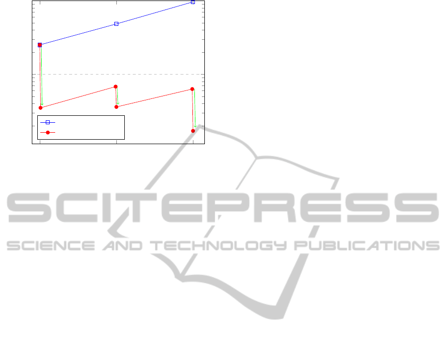
as shown in Figure 2.
CLOSER2015-5thInternationalConferenceonCloudComputingandServicesScience
448
100 200 300
10
2
10
3
251
484
965
35 36
68
63
17
Number of generations
Number of solutions
unrestricted bounds
adjustable bounds
Figure 2: Summary of results obtained in Experiment 2.
After 200 generations, the algorithm obtained a
total of 484 solutions with unrestricted bounds. Con-
sidering instead U
0
1
= 9000 [W], the algorithm only
found 68 solutions. The decision maker evaluated the
bounds associated to network traffic and adjusted the
upper bound U
2
to U
0
2
= 115 [Mbps], selecting only
36 of the 68 solutions (not considering 32 otherwise
feasible solutions) for the PF
reduced
.
Finally, after 300 generations, the algorithm ob-
tained a total of 965 solutions with unrestricted
bounds. Considering U
0
1
= 9000 [W] and U
0
2
= 115
[Mbps], the algorithm found 63 solutions. The de-
cision maker evaluated the bounds associated to eco-
nomical revenue and adjusted the lower bound L
3
to
L
0
3
= 13500 [$], selecting only 17 of the 63 solutions
(not considering 46 feasible solutions) for the final
PF
reduced
as shown in Figure 2. Clearly, at the end
of the iterative process, the decision maker found 17
solutions according to his preferences instead of the
untreatable number of 965 candidate solutions.
7 CONCLUSIONS AND FUTURE
WORK
This work proposed a general many-objective opti-
mization framework that is able to consider as many
objective functions as needed when solving the VMP
problem. As an example of utilization of the pro-
posed framework, for the first time a formulation of
the many-objective VMP problem (MaVMP) is pro-
posed, considering the simultaneous optimization of
the following five objective functions: (1) power con-
sumption, (2) network traffic, (3) economical revenue,
(4) quality of service and (5) network load balanc-
ing. In addition, a generalized multi-level of priori-
ties for the SLA associated to each VM is presented.
At the same time, constraints on upper and lower lim-
its of each objective function are also recommended
as a way to interactively control a potential explo-
sion in the number of non-dominated solutions, a well
known problem of many-objective optimization pro-
blems (von L
¨
ucken et al., 2014).
A short review of the most studied objective func-
tions was also presented to demonstrate that the num-
ber of objective functions may rapidly increase once
a complete understanding of the VMP problem is ac-
complished for practical problems were many diffe-
rent parameters should be ideally considered. Based
on the number of possible objective functions for
the VMP, this problem can clearly be addressed as a
many-objective optimization problem (MaOP).
Multiple challenges need to be considered for sol-
ving a many-objective optimization problem; there-
fore, an interactive memetic algorithm was proposed
to solve the proposed many-objective formulation,
validating the presented formulation and proving that
it is solvable. By no means, the authors claim that
the proposed interactive memetic algorithm is the best
way to solve this problem. This proposal only illus-
trates that it is possible to solve the problem although
the VMP problem becomes harder when increasing
the number of conflicting objective functions.
To validate the proposed algorithm, it was run
with different problem instances and experimental re-
sults were compared to the exact solution obtained
using an exhaustive search algorithm when possible.
In fact, the proposed algorithm found the complete
Pareto front and Pareto set (100%) for the 2 instan-
ces of Experiment 1. To validate the effectiveness
of the proposed algorithm reducing the increasing
number of non-dominated solutions obtained by the
Pareto dominance comparison, several problem ins-
tances were executed. In fact, considering the pro-
posed technique of interactively adjusting lower and
upper bounds associated to the values of each ob-
jective functions, the Pareto front could be reduced
from 965 original candidates to a treatable 17 non-
dominated solutions that satisfy the decision maker
preferences, as illustrated in Experiment 2.
At the time of this writing, the authors are working
on VMP formulations considering more complex net-
work topologies with full-duplex links. Considering
that this is the first formulation of the VMP problem
in a many-objective context, several future works can
be proposed considering all the already presented ob-
jective functions, studied so far in mono-objective as
well as multi-objective contexts.
Considering that this work proposed an offline
(static) formulation of the VMP problem in a many-
AMany-objectiveOptimizationFrameworkforVirtualizedDatacenters
449

objective optimization context, several challenges
need to be addressed for online (dynamic) formula-
tions of the problem, considering multi-objective and
many-objective approaches. At the same time, diffe-
rent meta-heuristics, methods and algorithms should
be still tested before a real good tool is ready for mas-
sive use in commercial cloud computing datacenters.
REFERENCES
Anand, A., Lakshmi, J., and Nandy, S. (2013). Virtual ma-
chine placement optimization supporting performance
slas. In Cloud Computing Technology and Science
(CloudCom), 2013 IEEE 5th International Confer-
ence on, volume 1, pages 298–305. IEEE.
B
´
aez, M., Z
´
arate, D., and Bar
´
an, B. (2007). Algorit-
mos mem
´
eticos adaptativos para optimizaci
´
on multi-
objetivo. In XXXIII Conferencia Latinoamericana de
Inform
´
atica–CLEI, volume 2007.
Barroso, L. A. and H
¨
olzle, U. (2007). The case for energy-
proportional computing. IEEE computer, 40(12):33–
37.
Beloglazov, A., Abawajy, J., and Buyya, R. (2012). Energy-
aware resource allocation heuristics for efficient man-
agement of data centers for cloud computing. Future
Generation Computer Systems, 28(5):755–768.
Beloglazov, A., Buyya, R., Lee, Y. C., Zomaya, A., et al.
(2011). A taxonomy and survey of energy-efficient
data centers and cloud computing systems. Advances
in Computers, 82(2):47–111.
Bin, E., Biran, O., Boni, O., Hadad, E., Kolodner, E. K.,
Moatti, Y., and Lorenz, D. H. (2011). Guarantee-
ing high availability goals for virtual machine place-
ment. In Distributed Computing Systems (ICDCS),
2011 31st International Conference on, pages 700–
709. IEEE.
Cheng, J., Yen, G. G., and Zhang, G. (2014). A many-
objective evolutionary algorithm based on directional
diversity and favorable convergence. In Systems,
Man and Cybernetics (SMC), 2014 IEEE Interna-
tional Conference on, pages 2415–2420.
Coello, C. C., Lamont, G. B., and Van Veldhuizen, D. A.
(2007). Evolutionary algorithms for solving multi-
objective problems. Springer.
Deb, K., Pratap, A., Agarwal, S., and Meyarivan, T. (2002).
A fast and elitist multiobjective genetic algorithm:
Nsga-ii. Evolutionary Computation, IEEE Transac-
tions on, 6(2):182–197.
Deb, K., Sinha, A., and Kukkonen, S. (2006). Multi-
objective test problems, linkages, and evolutionary
methodologies. In Proceedings of the 8th annual
conference on Genetic and evolutionary computation,
pages 1141–1148. ACM.
Donoso, Y., Fabregat, R., Solano, F., Marzo, J.-L., and
Bar
´
an, B. (2005). Generalized multiobjective multi-
tree model for dynamic multicast groups. In Commu-
nications, 2005. ICC 2005. 2005 IEEE International
Conference on, volume 1, pages 148–152. IEEE.
Farina, M. and Amato, P. (2002). On the optimal solution
definition for many-criteria optimization problems. In
Proceedings of the NAFIPS-FLINT international con-
ference, pages 233–238.
Gao, Y., Guan, H., Qi, Z., Hou, Y., and Liu, L. (2013). A
multi-objective ant colony system algorithm for vir-
tual machine placement in cloud computing. Journal
of Computer and System Sciences, 79(8):1230–1242.
L
´
opez Pires, F. and Bar
´
an, B. (2013). Multi-objective vir-
tual machine placement with service level agreement.
In Proceedings of the 2013 IEEE/ACM 6th Interna-
tional Conference on Utility and Cloud Computing,
pages 203–210. IEEE Computer Society.
L
´
opez Pires, F. and Bar
´
an, B. (2015). A virtual machine
placement taxonomy. In Proceedings of the 2015
IEEE/ACM 15th International Symposium on Cluster,
Cloud and Grid Computing. IEEE Computer Society.
Mishra, M. and Sahoo, A. (2011). On theory of vm
placement: Anomalies in existing methodologies and
their mitigation using a novel vector based approach.
In Cloud Computing (CLOUD), 2011 IEEE Interna-
tional Conference on, pages 275–282. IEEE.
Sato, K., Samejima, M., and Komoda, N. (2013). Dy-
namic optimization of virtual machine placement by
resource usage prediction. In Industrial Informatics
(INDIN), 2013 11th IEEE International Conference
on, pages 86–91. IEEE.
Shi, L., Butler, B., Botvich, D., and Jennings, B. (2013).
Provisioning of requests for virtual machine sets with
placement constraints in iaas clouds. In Integrated
Network Management (IM 2013), 2013 IFIP/IEEE In-
ternational Symposium on, pages 499–505. IEEE.
Shrivastava, V., Zerfos, P., Lee, K.-W., Jamjoom, H., Liu,
Y.-H., and Banerjee, S. (2011). Application-aware vir-
tual machine migration in data centers. In INFOCOM,
2011 Proceedings IEEE, pages 66–70. IEEE.
Sun, M., Gu, W., Zhang, X., Shi, H., and Zhang, W. (2013).
A matrix transformation algorithm for virtual machine
placement in cloud. In Trust, Security and Privacy
in Computing and Communications (TrustCom), 2013
12th IEEE International Conference on, pages 1778–
1783. IEEE.
Tom
´
as, L. and Tordsson, J. (2013). Improving cloud infras-
tructure utilization through overbooking. In Proceed-
ings of the 2013 ACM Cloud and Autonomic Comput-
ing Conference, CAC ’13, pages 5:1–5:10, New York,
NY, USA. ACM.
von L
¨
ucken, C., Bar
´
an, B., and Brizuela, C. (2014). A
survey on multi-objective evolutionary algorithms for
many-objective problems. Computational Optimiza-
tion and Applications, pages 1–50.
CLOSER2015-5thInternationalConferenceonCloudComputingandServicesScience
450
