
Comfort-constrained Demand Flexibility Management for Building
Aggregations using a Decentralized Approach
L. A. Hurtado, E. Mocanu, P. H. Nguyen, M. Gibescu and W. L. Kling
Department of Electrical Engineering, Eindhoven University of Technology,
5600MB, Eindhoven, The Netherlands
Keywords:
Demand Flexibility, Resource Allocation, Demand Side Management, Building Energy Management System,
Energy Management.
Abstract:
In the smart grid and smart city context, the energy end-user plays an active role in the operation of the power
system. The rapid penetration of Renewable Energy Sources (RES) and Distributed Energy Resources (DER)
requires a higher degree of flexibility on the demand side. As commercial and Industrial buildings (C&I)
buildings represent a substantial aggregation of loads, the intertwined operation of the electric distribution
network and the built environment is to large extent responsible for achieving energy efficiency and sustain-
ability targets. However, the primary purpose of buildings is not grid support but rather ensuring the comfort
and safety of its occupants. Therefore, the comfort level needs to be included as a constraint when assessing
the flexibility potential of the built environment. This paper proposes a decentralized method for flexibility
allocation among a set of buildings. The method uses concepts from non-cooperative game theory. Finally,
two case of study are used to evaluate the performance of the decentralized algorithm, and compare it against a
centralized option. It is shown that flexibility requests from the grid operator can be met without deteriorating
the comfort levels.
1 INTRODUCTION
Traditionally, electricity demand is considered un-
controllable, however, relatively well predictable in
a certain aggregation level. Thus, power generation
needs simply to follow the load at all times. Imbal-
ances between supply and demand might come from
unforeseen demand fluctuations and generation units
failures. To deal with possible system imbalances,
transmission system operators (TSOs) make use of
automated, i.e. primary and secondary control, or
manual, i.e. tertiary control, power reserves (Entso-
e, 2004; Ulbig and Andersson, 2012). This capacity
of the system to react and adapt in a tolerable time to
these unforeseen events is known as flexibility.
With the introduction of renewable energy sources
(RES), distributed energy resources (DER) like stor-
age, and the new type of loads like electric vehicles
(EVs), new forms of uncertainty are introduced to the
power system operation. These lead to more frequent
system problems, e.g. generation-demand mismatch,
and network problems, e.g. voltage stability, network
congestion, blinding of protecting devices, etc. To
deal with these challenges the active and smart con-
trol of the demand domain is required (Kefayati and
Baldick, 2012). Recently, a considerable amount of
attention has been given to the concept of “demand
flexibility”. Conventionally, flexibility was harnessed
from power generation units. However, the flexibility
offered by the end-users has the potential to help not
only resolve network problems, but also accommo-
date a higher amount of RES, increase asset utiliza-
tion and reduce peak demand (Morales-Vald
´
es et al.,
2014; Kirschen et al., 2012; Ulbig and Andersson,
2012).
Generally, the use of flexible demand for system
and network support activities can be grouped under
Demand Side Management (DSM) and Demand Re-
sponse (DR) activities. Roughly, DSM refers to the
long-term and short-term measures designed to influ-
ence the consumption pattern in such a way that it
will influence the load shape of the utility, i.e. distri-
bution system operator (DSO). Whereas, DR refers to
the mechanisms designed to directly influence the de-
mand of consumers in response to supply conditions,
for instance through the use of market prices (Lam-
propoulos et al., 2013; Gellings, 2009). Literature
shows that the smart management of flexible loads
can indeed support grid operation and offer ancillary
system services, without compromising the primary
157
Hurtado L., Mocanu E., Nguyen P., Gibescu M. and Kling W..
Comfort-constrained Demand Flexibility Management for Building Aggregations using a Decentralized Approach.
DOI: 10.5220/0005444101570166
In Proceedings of the 4th International Conference on Smart Cities and Green ICT Systems (SMARTGREENS-2015), pages 157-166
ISBN: 978-989-758-105-2
Copyright
c
2015 SCITEPRESS (Science and Technology Publications, Lda.)

Nomenclature:
i Index for wall, window, roo f
k Index for H
2
O, CO
2
A
i
Area of i, [m
2
]
c
p,a
Heat capacity of air, [kJ/KgK]
c
p,i
Heat capacity of i, [kJ/KgK]
c
p,w
Heat capacity of water, [kJ/KgK]
η
f an
Rated fan efficiency
Flex
d
Requested flexibility, [%]
Flex
s
Offered flexibility, [%]
Flex
a
flexibility of the aggregator, [%]
γ
air
Specific weight of air, [N/m
3
]
M
i
Mass of i, [Kg]
M
air
Mass of the building air volume, [Kg]
M
CO
2
CO
2
molecular weight, [gr/gr
mol
]
N Occupancy
Q
gen
Metabolic heat rate, [J/hr]
P
z
Building pressure, [atm]
Φ
k
env
concentration of k in outdoor air, [gr/hr]
Φ
gen,k
Metabolic generation rate of k,
gr
k
/m
3
Φ
k
humid
Humidifier mass removal rate of k, [gr/hr]
V
Z
Space volume, [m
3
]
H
lat
Latent heat of condensation, [kJ/gr
H
2
O
]
H
rated
Rated head of the fan, [m]
R Universal gas constant, [atm m
3
/gr
mol
K]
ρ
i
Density of i,
Kg/m
3
ρ
w
Density of water,
Kg/m
3
T
env
Temperature of return water, [K]
T
r,w
Temperature of supplied water, [K]
T
s,w
Temperature of supplied water, [K]
T
s,a
Temperature of supplied air, [K]
U
i
Heat transfer coefficient of i,
kJ/hr m
2
K
˙v
s,w
water supply flow rate, [m
3
/s]
˙v
s
Air supply flow rate, [m
3
/s]
˙v
r
Air removal flow rate, [m
3
/s]
˙v
in
Outdoor air supply flow rate, [m
3
/s]
˙v
out
Exhaust air flow rate, [m
3
/s]
˙v
rated
Rated fan speed, [m
3
/s]
mission of the controlled loads (Schl
¨
osser et al., 2014;
Baccino et al., 2014; Cheng et al., 2014). In (Morales-
Vald
´
es et al., 2014) the effect of comfort relaxation
on the energy demands of buildings is presented. In
(Hurtado et al., 2014) the effect of different build-
ing operation scenarios on a low voltage distribution
network is assessed. In (Klaassen et al., 2013) the
potential of DSM in the perspective of the DSOs is
discussed. In (Kobus et al., 2015) the role of smart
appliances in the real electricity demand shift is pre-
sented, in the Dutch context. In (Sajjad et al., 2014)
the effective use of demand flexibility for peak re-
duction is discussed, in a residential customers con-
text. However, throughout literature the correlation
between comfort and demand flexibility, in the con-
text of grid support is still lacking. Furthermore, flex-
ible resources can be allocated and managed in a sim-
ilar way as generation resources using market-based
approaches, e.g. constrained economic dispatch, or
heuristic approaches, e.g. genetic algorithms, to meet
a flexibility demand (Berardino et al., 2012; Gupta
et al., 2012).
As demand flexibility is a scarce resource that
needs to be assigned to various uses, it requires aggre-
gation to have a noticeably positive impact on the grid
operation. Buildings differ in size, functions, energy
demand and are under constant change. They consist
of different systems that differ in dynamics and life
time. However, their main function is to provide oc-
cupants with a comfortable and healthy indoor envi-
ronment, i.e. about 50% of the total electrical energy
consumed by the building, is used for comfort man-
agement (Zhao et al., 2013). Therefore, to guarantee
the correct operation of both systems, i.e. electricity
grid and building, not only network constraints but
also comfort constraints should be included in the al-
location of flexibility obligations.
In this paper, comfort is proposed as a necessary
metric for demand flexibility in the built environment.
As the building objective is different from grid sup-
port, comfort needs to be monitored and constrained
when offering flexibility. A straightforward building
energy and comfort model is developed in this pa-
per to represent the dynamics of building operation,
while establishing a relationship between comfort and
energy management. Here, only flexibility from the
comfort systems is considered, not only because it
represents a great part of the total energy consumed
by the building, but also because there is a time lapse
between comfort variation perception and the comfort
system operation, which allows for such systems to
be operated in non traditional ways. Furthermore, we
propose the use of a n-player non-cooperative game
to allocate a flexibility request over a finite number
of buildings, without violating the comfort limits for
each of the buildings. This is a decentralized ap-
proach that reduces the need for the aggregation of
information to achieve an optimal solution. Finally,
using the building model proposed, two case studies
are used to evaluate the performance of the proposed
decentralized algorithm.
The remainder of this paper is divided into 5 sec-
tions. In the next section the flexibility inherent to the
built environment is discussed in terms of power and
comfort demand. Furthermore, in this section the en-
velope model of a building is presented. This model
is used to represent the comfort and energy dynamics
of each player in the game. In the following section
the aggregator’s role is introduced. In section 4 the
SMARTGREENS2015-4thInternationalConferenceonSmartCitiesandGreenICTSystems
158

case study consisting of 5 buildings is presented, with
the numerical results. Finally, section 5 summarizes
and presents conclusions from this work.
2 FLEXIBILITY IN THE BUILT
ENVIRONMENT
Being responsible for about one-third of the energy
consumed in cities (Park et al., 2011), commercial
and industrial (C&I) buildings have the potential to
significantly contribute to the efficient operation of
the power system, accommodate a higher amount of
RES, increase asset utilization and reduce peak de-
mand (Hurtado et al., 2014; Morales-Vald
´
es et al.,
2014; Kirschen et al., 2012; Ulbig and Andersson,
2012). However, the main objective of building is far
from being either system or network support. In gen-
eral, building operation involves comfort and energy
management tasks. Roughly, comfort management
represents more than half of the total building energy
demand (Zhao et al., 2013). This means that flexibil-
ity, if defined as the demands’s capability to react and
adapt in a tolerable time to unforeseen system or net-
work events, will potentially have a negative impact
on the building comfort.
As mentioned, the first main task of a building
management system is comfort management. How-
ever, comfort is a complex and subjective human per-
ception. In previous work, the authors conceptual-
ized comfort as a function of both thermal and air
quality while CO
2
concentration levels were kept as
a system constraint (Hurtado et al., 2014). Tradition-
ally, temperature and relative humidity are used as the
metrics to represent thermal and air quality comfort.
In (1) comfort is described as a combination of two
Gaussian functions representing thermal and air qual-
ity comfort.
com f = (ω)e
−(T −µ
T
)
2
2σ
2
T
| {z }
Thermal comfort
+(1 − ω)e
−(Rh−µ
RH
)
2
2σ
2
Rh
| {z }
Air quality comfort
(1)
where, ω is a weight factor; T is the building’s tem-
perature; µ
T
is the mean temperature value, or the op-
timal temperature set point; σ
T
is the thermal comfort
standard deviation, which represents the discomfort
tolerance; Rh is the relative humidity; µ
RH
is the mean
humidity, or air quality optimal set point; and σ
RH
is
the standard deviation for air quality comfort, which
represents the discomfort tolerance.
The second main task of a building management
system is energy management. This work categorizes
the energy systems of a building into comfort and
non-comfort systems. Energy demand of a comfort
system corresponds to the energy consumed for com-
fort management. Whereas, the energy demand of a
non-comfort systems correspond to specific individ-
ual systems in local zones.
The total power consumption, in watts [W ], of a
building is expressed in the following equation:
P
total
=
z
∏
i=1
P
AHU
+ P
heater
| {z }
comfort
+
z
∑
i=1
P
i
|{z}
non-comfort
(2)
where, P
AHU
represents the power demand of the Air
Handling Unit (AHU) for air quality comfort; P
heater
is the power consumed by the heating system for ther-
mal comfort purposes; and P
i
represents the power
consumed by the zone’s devices in the Z zones, e.g.
lights, computers, etc.
2.1 The Envelope Model
A building is a complex multi-zonal comfort system,
governed by the energy and mass conservation princi-
ples. In the context of the smart grid and smart cities,
for the built environment flexibility to have a notice-
able positive impact on the grid operation, aggrega-
tion is required. This process requires irrelevant in-
formation to be neglected and the simplification of the
models used. Thus, in the same context, it is impracti-
cal and highly complex to have a detail, zone by zone,
model of the building. In this work an envelope model
is developed, in which the building is represented as a
single zone system. Such model gives a fair approxi-
mation to the energy and comfort dynamics of a build-
ing. In this model, there are three state variables: the
zone temperature (T ), the zone relative humidity (Rh)
and the zone CO
2
concentration (Φ
CO
2
) levels. More-
over, the air in the zone is assumed to be fully mixed,
i.e. uniform temperature distribution, with constant
density, and the pressure losses in the zone and the
effect of the building orientation, i.e. solar gains, are
neglected. Finally, occupancy (N) and the weather,
i.e. temperature (T
env
), water concentration (Φ
H
2
O
env
),
and CO
2
concentration (Φ
CO
2
env
), are the uncontrolled
inputs.
2.1.1 Thermal Dynamics
With the aforementioned assumptions, the thermal
dynamics of the building represented through lumped
capacity model described by the energy conservation
principle:
dT (t)
dt
=
1
M
air
c
p,a
(Q
in
+ Q
heater
− Q
loss
) (3)
Comfort-constrainedDemandFlexibilityManagementforBuildingAggregationsusingaDecentralizedApproach
159

where, Q
in
represents the internal gains due to the heat
generation of occupants; Q
heater
represents the heat
contribution of the heating system used. Finally, Q
loss
is used to model the heat losses through the envelope
of the zone.
The energy transferred to the building is propor-
tional to the energy transferred by the heating system,
as expressed in (4), and by heat contribution of the
occupants, as expressed in (5).
Q
heater
= ˙v
s,w
ρ
w
c
p,w
(T
s,w
− T
r,w
) (4)
Q
in
= N Q
gen
(5)
The energy removed from the building is the en-
ergy lost to the environment through the building en-
velope. These are represented through the conduction
and convective heat transfer mechanisms,
Q
loss
=
n
∑
i=1
U
i,in
A
i
(T
i
− T ) (6)
where, n is number of envelope elements, and their
temperature, T
i
, is given by:
dT
i
(t)
dt
=
U
i,in
A
i
(T − T
i
) +U
i,out
A
i
(T
i
− T
env
)
M
i
c
p,i
(7)
where, T
env
is the outdoor air temperature.
2.1.2 Air Quality Dynamics
Air is a mixture of multiple elements in different con-
centrations. Indoor air quality is traditionally mea-
sured through the water content, i.e. relative humidity,
and CO
2
concentration dynamics in the air. These dy-
namics can be represented through the mass and com-
ponent balances in the air volume. The concentration
change in time of an element k is proportional to the
particles of that element added and extracted from the
volume, as expressed in the following equation:
dΦ
k
dt
=
1
V
z
˙v
s
Φ
k
s
− ˙v
r
Φ
k
+ NΦ
gen,k
(8)
where, the concentration of element k in the supplied
air, Φ
k
s
, is given by:
Φ
k
s
=
1
˙v
s
˙v
r
Φ
k
+ ˙v
in
Φ
k
env
− ˙v
out
Φ
k
+ Φ
k
humid
(9)
where, Φ
k
env
is the concentration of k in the outdoor
air, and Φ
k
humid
is the humidifier mass removal rate of
element k, with Φ
k
humid
= 0, ∀ k = CO
2
.
Finally, using the Ideal gas law, relative humid-
ity and the CO
2
concentration can be rewritten as fol-
lows:
Rh(t) = 100
Φ
H
2
O
Φ
sat
H
2
O
(10)
[ppm]Φ
CO
2
= 1000
Φ
CO
2
R T
z
M
CO
2
P
z
(11)
where, the saturated concentration of water is given
by Antoine’s equation:
Log
10
(Φ
sat
H
2
O
) = 8.07131 −
1730.63
T − 39.73
(12)
2.1.3 Energy Dynamics
As mentioned, a large part of the building’s energy de-
mand comes from the comfort management systems.
In this section, and for the rest of the paper, we con-
sider only the AHU and heating system as the flexibil-
ity sources of the building. These systems aim to keep
the comfort parameters within the designed ranges,
according to the dynamics previously described. In a
general way, the energy consumed by these systems
is used to move and heat up the water (P
heater
), and
the air (P
AHU
) in the building.
The electrical power consumed by the heating sys-
tem is proportional to the ratio between the system’s
heat output and its coefficient of performance COP,
which is used to describe the ratio between the useful
heat produced and the power input.
P
heater
=
Q
heater
COP
(13)
where, Q
heater
is given by (4) as a function of the zone
temperature T .
Before new air is added to the building, it goes
through several steps. These can be summarized in
three general steps: air mixing, air pre-heating or pre-
cooling, and air humidification. In the first step, the
return air is mixed with new air from the outside, this
process helps to control the particles concentration in
the air to be supplied back to the zone. In the sec-
ond step, the mixed air is heated up or cooled down
to the desired temperature. This is done by the action
of the heating and cooling elements of the AHU. In
the last step, water is added to the air to control the
humidity of the supply air. The electrical power con-
sumed by the AHU to control the quality of the air
in the building is proportional to the power consumed
to move the air in and out the zone, to condition the
air to the right temperature, and to humidify the air to
the desired value. In the envelope model used in this
work, this corresponds to the power consumed by the
fan, heating and humidifying systems of the AHU, as
expressed in the following equation:
P
AHU
= P
f an,s
+ P
f an,r
+ P
coil
+ P
lat
(14)
where, P
f an,s
, P
f an,r
, P
coil
and P
lat
depend on the var-
ious air flow and mass removal rates used to control,
both the water and CO
2
concentrations rates given by
SMARTGREENS2015-4thInternationalConferenceonSmartCitiesandGreenICTSystems
160

(8), and according to the following equations:
P
f an
=
γ
air
( ˙v
f an
)
3
H
rated
η
f an
( ˙v
rated
)
2
(15)
P
coil
=
˙v
in
c
p,a
(T
s,a
− T
mix
)
COP
coil
(16)
P
lat
= Φ
H
2
O
humid
H
lat
(17)
where, ˙v
f an
is the air flow going through the fan, i.e.
˙v
in
for the supply fan, and ˙v
out
for the return fan. Fi-
nally, T
mix
is the temperature of the air in the mixing
room, and it is given by:
T
mix
=
(( ˙v
in
− ˙v
out
)T
env
+ ˙v
out
T )
˙v
in
(18)
3 FLEXIBILITY AT THE
AGGREGATOR LEVEL
Despite C&I buildings being a considerable load
to the power system, they are by themselves not
big enough to have a noticeable positive impact
on the grid operation. This creates the need for an
aggregating entity, with the role of accumulating
flexibility to meet a request from the grid at the
lowest comfort cost (Backers et al., 2014). Here,
flexibility [%] is conceptualized as the ratio between
flexible power, and the total power demand at a
given moment of time. For instance, the building’s
flexibility, i.e. (Flex
s
), is defined as the ratio between
the building’s flexible power, and the building’s peak
power. The grid’s flexibility request, i.e. (Flex
d
),
is defined as the ratio between the change in power
required, and the total power demanded in the grid.
In general, an aggregating entity aims to distribute the
grid’s flexibility request, (Flex
d
), over a portfolio of
buildings, each with its own flexibility offer (Flex
s
).
Such problem is analogue to a constrained resource
allocation problem with a hard comfort constraint, as
described next:
Minimize
∆ Flex = Flex
d
−
B
∑
j=1
Flex
s, j
(19)
Subject to
com f
j
≥ com f
j,min
(20)
However, this requires the aggregating unit to
have knowledge over the building dynamics and the
effect of flexibility on the building comfort. Nonethe-
less, the aggregator resources are owned and managed
by different entities, with different objectives, users
and priorities. In the scope of this arguments, let
us introduce the concept of a non-cooperative game
and develops methods for the mathematical analyse
of such game. The game presented is a n-person game
defined by means of pure strategies and pay-off func-
tions defined for the combinations of pure strategies.
At the aggregated level a multi-player game is in-
vestigated in order to find a optimum flexibility point
under a equal comfort condition in a different number
of buildings. This full decentralized solution is used
to compute one sample Nash Equilibrium point. Nash
proved that this equilibrium concept exists for any
game with a finite number of players, each of them
having a finite number of strategies (Nash, 1951).
In a classical normal form, the optimization
formulation of n-person non-cooperative games,
Γ(B,Flex
s
,R), consists of the following:
• A set B = {1,..., j} of buildings (players).
• A finite set Flex
( j)
s
of strategies for each
building j ∈ B, were Flex
s
is defined by a
set of n-tuples of pure strategies, such as
(Flex
0
,Flex
10
,Flex
20
,Flex
30
,Flex
50
).
• A reward (pay-off) function, R
j
: Flex
s
→ R, for
each building j ∈ B, which maps the set of all n-
tuples of pure strategies into the real numbers.
The payoff function (R
j
) has a unique ex-
tension to the n-tuples of mixed strategies which
is linear in the mixed strategy of each player,
R
j
(Flex
(1)
s
,...,Flex
(B)
s
).
Theorem 1. (Nash, 1951) The mixed extension of the
finite game Ω(B, Flex
s
,R) has at least one strategic
equilibrium.
Formally, a n-tuple Ω is an equilibrium point if
and only if for every j
R
j
(Ω) = max
∀γ
j
,ψ
[R
j
(Ω;γ
j
)] (21)
where Ω = (Flex
(1)
s
,...,Flex
(B)
s
). Thus, an equilib-
rium point is a n-tuple Ω such that each player’s
mixed strategy maximizes his payoff if the strate-
gies of the others are held fixed. Thus, each player’s
strategy is optimal against those of the others. A
mixed strategy Flex
( j)
s
use a pure strategy Π
jα
if
ψ
j
=
∑
α
c
jα
Π
jα
and c
jα
> 0. From the linearity of
R
j
(Flex
(1)
s
,...,Flex
(B)
s
) in ψ
j
max
∀γ
j
,ψ
[R
j
(Ω;γ
j
)] = max
α
[R
j
(Ω;Π
jα
)] (22)
Let R
jα
(Ω) be defined as R
jα
(Ω) = R
j
(Ω;Π
jα
).
Then, the following necessary and sufficient condi-
tion for Ω to be an equilibrium point is:
R
j
(Ω) = max
α
R
jα
(Ω) (23)
Comfort-constrainedDemandFlexibilityManagementforBuildingAggregationsusingaDecentralizedApproach
161
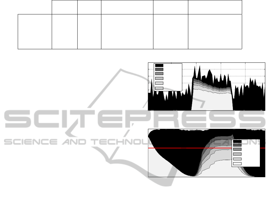
Table 1: Building envelope characteristics.
Volume Area Occupancy Peak power Non-flexible power
[m
3
] [m
2
] N
av
t
in
t
out
[kW ] [kW ]
Building A 4536 453.6 20 7hr 18hr 8.18 2.45
Building B 18144 1814.4 37 9hr 14hr 12.6 3.78
Building C 10206 1020.6 30 9hr 17hr 10.08 3.02
Building D 1134 113.4 14 12hr 20hr 7.56 2.26
Building E 2268 226.8 10 8hr 17hr 7.57 2.27
An equivalent condition for every j and α is:
R
j
(Ω) − R
jα
(Ω) ≥ 0 (24)
More generally, the set of all equilibrium strate-
gies ψ
B
are simply the set of good strategies of a
player which is a convex polyhedral subset of his
mixed strategy space. A strong solution exists only
when there is a saddle point in the pure strategies.
In (24) an equivalent form of the non-linear flexibil-
ity optimization problem defined in (19) is presented,
where R
(.)
' Flex
(.)
.
This problem has been discussed in the literature
in different forms. In the case of cooperative games,
the players (agents) exchange information between
them, and in the case of non-cooperative games the
players do not exchange information, to achieve the
same Nash equilibrium point. A more comprehen-
sive discussion can be found in (Khan and Sun, 2002;
Rosenthal, 1989), and some examples of different ap-
plications for the non-cooperative games can be seen
in (Chatterjee, 2009; Fadlullah et al., 2011).
4 CASE STUDY
Using the building model described in section 2, we
evaluate the performance of n-person non-cooperative
game, and experimentally it is shown that the flexibil-
ity request can be met by providing efficient flexibility
schedules, while comfort is kept within the required
boundaries.
Five different buildings are modelled. The major
differences between these five simulated buildings are
summarized in Table 1. Each building has three main
state variables, the zone temperature (T ), the zone rel-
ative humidity (Rh) and the zone CO
2
concentration
(Φ
CO
2
) levels. These variables do not only relate to
to the comfort, but also to the energy behaviour of the
building model, as described in section 2. Different
occupancy profiles were used for each building. Each
building has an average number of occupants N
av
with
a random variation in time (see Table 1), as expressed
in the following equation:
5 10 15 20
0
2
4
6
8
10
12
14
Power [kW]
time [hrs]
Building load profile
No energy Opt
Energy Opt
flex
s
=10%
flex
s
=20%
flex
s
=30%
flex
s
=50%
0 5 10 15 20
0
20
40
60
80
100
Occupant satisfaction [%]
time [hrs]
Building comfort profile
No energy Opt
Energy Opt
flex
s
=10%
flex
s
=20%
flex
s
=30%
flex
s
=50%
Figure 1: Example building load and comfort profile.
N =
N (N
av
,1) if t
in
< t < t
out
0 if t ≤ t
in
∨ t ≥ t
out
(25)
Moreover, the building behaviour is also weather
dependant. The model uses simulated weather data
for temperature, water and CO
2
concentration in air,
representing a typical winter day in The Netherlands.
In a first simulation, the peak power for every building
is obtained, as summarized in Table 1. Consequently,
varying the flexibility offer of each building, Flex
s
,
the building behaviour is obtained for every building.
Figure 1 is given as an example to illustrate such be-
haviour of a building. The upper figure shows the
building power demand for different flexibility offers,
and the bottom figure shows the occupant satisfaction,
i.e. comfort, as depicted in (1). This figure shows that
as the flexibility offer is increased, the building com-
fort profile is deteriorated.
The grid flexibility request, an hourly reduction
request, is set to vary between 0 and 50% of the total
flexible power offered by the aggregator. This is the
accumulated flexibility from the aggregator’s portfo-
lio, Flex
a
=
∑
B
j=1
Flex
s, j
. In a similar way, buildings
are allowed to provide up to half of their flexible
SMARTGREENS2015-4thInternationalConferenceonSmartCitiesandGreenICTSystems
162

Algorithm 1: N-player game algorithm.
%Initialization
Buildings → Players
Building flexibilities → Actions
%Get buildings’ flexibility response
for all time steps do
for all SmartGrid flexibilities requests do
for all (p,a)∈(Players, Actions) do
initialize rewards R(p,a)
end for
PlayGame(Players,Actions,R)
Nash equilibrium → Buildings’ response
end for
end for
power, i.e. Flex
s
∈ {10%, 20%,30%, 50%}. For an
arbitrary number of buildings, the demand flexibility
resource allocation problem can be solved using the
pseudo-code from Algorithm 1 and playing a n-player
game as described in Section 3.
The proposed solution seeks the right balance be-
tween, the request made by the smart grid, and the
flexibility available in buildings. In this solution, each
building commits discrete parts of their flexible power
as a flexibility offer, Flex
s
, relative to the flexibility
request, Flex
d
.
In the remaining of this paper we present two test
cases which involve two and five buildings, respec-
tively. In both cases, we ensure the end-user comfort
to be within the limit, i.e. com f
min
> 60%, which ac-
cording to the definition presented earlier in (1), cor-
responds to the upper and lower comfort limits estab-
lished by ASHRAE Standard 55-1992.
4.1 Case 1: 2-player Game
In this first case the n-person games is played between
two of the five buildings. Buildings D and E are se-
lected for this first case, since they are the smallest
buildings, but they also showed the most different oc-
cupancy profiles. This means, that these two buildings
are able to supply more flexibility with a lower impact
on their comfort profiles. The exact results obtained
for various smart grid flexibility requests are shown
in Table 2 and Figure 2. As mentioned, the building
results are presented as percentages of the total flex-
ibility request. For instance, if the Smart Grid flexi-
bility request is 10% of the current electricity demand
at midnight, i.e. time = 24h, the flexibility offer of
buildings D and E is 47.9% and 80.4% respectively.
In this case, the buildings can offer higher demand
flexibility than that requested by the grid. However,
as the flexibility request is increased, the building’s
offer start to decrease in relation to the request (see:
Table 2: Flexibility response under different Smart Grid re-
quests, as percentage of the total flexibility request
Smart Grid flexibility request at the aggregated level
10% 20% 30% 40% 50%
Time Buildings flexibility response [%]
[h] D E D E D E D E D E
1 0 0 0 0 163.4 163.4 122.5 122.5 98.0 98.0
2 297.7 0 148.8 0 99.2 0 74.4 0.0 59.5 0
3 0 0 0 0 0 0 0 0 0 0
4 0 0 0 0 0 0 0 0 0 0
5 0 0 121.6 0 81.1 0 60.8 0 48.6 0
6 180.4 0.0 90.2 0 60.1 0 45.1 0 36.1 0
7 84.7 0 42.3 0 28.2 0 21.2 0 16.9 0
8 93.1 0 46.6 0 31.0 0 23.3 175.7 18.6 140.5
9 0 191.9 0 95.9 0 64.0 151.6 48.0 121.3 38.4
10 0 0 0 150.8 0 100.5 0 75.4 0 60.3
11 0 0 0 0 0 0 0 181.8 0 145.4
12 0 0 0 0 0 0 0 0 0 0
13 0 0 0 0 0 0 0 180.2 0 144.2
14 0 100.3 0.0 50.1 0.0 33.4 0 25.1 0 20.1
15 0 0 0 140.8 0 103.6 0 77.7 56.8 62.2
16 0 0 0 107.9 0 79.7 0 59.8 61.4 47.8
17 0 158.1 0 91.0 0 60.7 0 45.5 0 36.4
18 0 46.0 0 23.0 0 15.3 148.2 11.5 118.6 20.7
19 0 117.9 0 81.4 0 54.3 0 40.7 0 32.6
20 0 0 0 0 0 0 0 0 0 0
21 0 0 0 0 0 0 0 0 0 0
22 127.1 85.5 74.0 42.7 49.3 28.5 37.0 21.4 29.6 17.1
23 0 0 0 0 0 0 0 0 0 0
24 47.9 80.4 24.0 40.2 16.0 26.8 12.0 20.1 9.6 16.1
Table 2). Finally, from the Figure 2 it can be seen
that the aggregator is able to meet the grid request
while ensuring that the comfort of both buildings is
kept higher than 60%.
Additionally, in figure 3, we compared the de-
centralized Dynamic Game Theory (DGT) approach
against a centralized approach using Particle Swarm
Optimization (PSO). At the aggregated level PSO is
used to allocate the flexibility obligations among the
Figure 2: Flexibility responses averaged over a day for 2
buildings under different grid flexibility requests, with mean
and standard deviation.
Comfort-constrainedDemandFlexibilityManagementforBuildingAggregationsusingaDecentralizedApproach
163
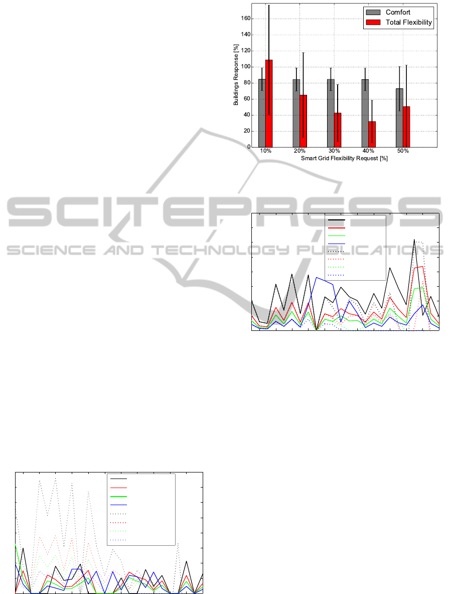
playing buildings. In (Hurtado et al., 2014) more de-
tails and the mathematical description of the PSO ap-
proach can be found. In the figure the playing buil-
ings’ aggregated flexibility is shown as a percentage
of the flexibility request. It is observed that the cen-
tralized approach offers higher flexibility during the
morning hours. However, the decentralized approach
offers better results during the afternoon hours, time
in which both buildings are occupied.
4.2 Case 2: 5-player Game
In the second case study the n-person non-cooperative
game is played between the 5 buildings (i.e. A, B, C,
D, and E). In Table 3 the exact results as percentages
of the flexibility request at the aggregated level are
presented for the various grid requests. As before, ev-
ery building is allowed to give up to 50% of its own
flexible power on an hourly basis, and this is in some
cases, is higher than the grid request. In Figure 4 the
effect on comfort is also presented. It can be observed
how the increase of the flexibility request has a nega-
tive effect on the overall comfort level of the building.
It can also be seen that the total relative flexibility of-
fer is decreased as the request increases. However,
from the table it can be observed that as the request is
increased, the number of buildings participating in the
flexibility offer increases. From the table it can also
been seen that for most of requests buildings B and
C do not offer flexibility. Despite being the bigger
buildings, i.e. higher peak load, the relation between
comfort and flexibility is worst for these two build-
ings. For instance, Figure 1 shows such relation for
the building C.
It is worth highlighting, that in some cases the
buildings provide a flexibility response over one
hundred percent. This happens due to the fact
that the grid requests and buildings response is dis-
cretized and we work with fixed flexibility points, i.e.
Flex
( j)
s
∈ {10%,20%,30%, 50%}. This can be used
2 4 6 8 10 12 14 16 18 20 22 24
0
100
200
300
400
500
600
700
800
Time [h]
Buildings’ flexibility response [%]
Flex 10% DGT
Flex 20% DGT
Flex 30% DGT
Flex 50% DGT
Flex 10% PSO
Flex 20% PSO
Flex 30% PSO
Flex 50% PSO
Figure 3: Centralized (PSO) versus decentralized (DGT)
buildings’ D and E flexibility response.
Figure 4: Flexibility and comfort profile responses averaged
over a day for all 5 buildings relative to different grid flexi-
bility requests, with mean and standard deviation.
2 4 6 8 10 12 14 16 18 20 22 24
0
50
100
150
200
250
300
350
400
Time [h]
Buildings’ flexibility response [%]
Flex 10% DGT
Flex 20% DGT
Flex 30% DGT
Flex 50% DGT
Flex 10% PSO
Flex 20% PSO
Flex 30% PSO
Flex 50% PSO
Figure 5: Centralized (PSO) versus decentralized (DGT)
buildings’ flexibility response.
as an advantage to shift the load to time periods where
the Smart Grid flexibility request can not be fulfilled.
One solution for this, can be achieved by adjusting
dynamically the flexibility games.
In figure 5, we compared again the decentralized
DGT approach against the centralized approach PSO.
It is observed that in the first 7 hours and in the last
hours of the day both methods offer similar solutions.
This is mainly due to the fact that during these periods
the buildings are mostly unoccupied. Moreover, it is
also observed that the decentralized solution has in
general better results than the centralized one.
5 CONCLUSIONS
This paper proposed a decentralized algorithm for
flexibility request allocation among an aggregated
portfolio of buildings. Furthermore, the use of com-
fort as a metric for flexibility in the built environment
SMARTGREENS2015-4thInternationalConferenceonSmartCitiesandGreenICTSystems
164

Table 3: Flexibility response under different Smart Grid requests, as percentage of the total flexibility request.
Smart Grid flexibility request at the aggregated level
Flexibility request [10%] Flexibility [20%] Flexibility [30%] Flexibility [40%] Flexibility [50%]
Time Building flexibility response
[h] A B C D E A B C D E A B C D E A B C D E A B C D E
1 0 0 0 102.4 0 0 0 0 51.2 0 0 0 0 34.1 0 0 0 0 25.6 0 0 0 0 20.4 0
2 0 0 0 29.5 0 0 0 0 14.7 0 0 0 0 9.8 0 0 0 0 7.3 0 0 0 0 5.9 0
3 0 0 0 23.2 0 0 0 0 11.6 0 0 0 0 7.7 0 0 0 0 5.8 0 0 0 0 4.6 0
4 0 0 0 123.5 34.5 0 0 0 61.7 17.2 0 0 0 41.1 11.5 0 0 0 30.8 8.6 0 0 0 24.7 6.9
5 0 0 0 28.8 39.4 0 0 0 14.4 19.7 0 0 0 9.6 13.1 0 0 0 7.2 9.8 0 0 0 5.7 7.8
6 0 0 0 149.24 42.5 0 0 0 74.6 21.2 0 0 0 49.7 14.1 0 0 0 37.3 10.6 0 0 0 29.8 8.5
7 0 0 0 0 57.0 0 0 0 0 28.5 0 0 0 0 19.0 0 0 0 0 14.2 0 0 0 0 11.4
8 0 0 0 0 188.6 0 0 0 0 94.3 0 0 0 0 62.8 0 0 0 0 47.1 0 0 38.0 10.6 37.7
9 0 0 0 0 0 0 0 0 0 0 0 0 0 0 0 0 0 0 0 0 19.5 75.6 60.1 3.0 21.8
10 0 0 0 0 114.6 0 0 0 0 57.3 0 0 0 0 38.2 0 0 0 0 28.6 21.6 65.9 55.7 2.0 22.9
11 0 0 0 0 94.1 0 0 0 0 47.0 0 0 0 0 31.3 0 0 0 0 23.5 8.7 68.2 48.2 12.59 18.8
12 0 0 0 98.8 48.7 0 0 0 49.3 24.3 0 0 0 32.9 16.2 0 0 0 24.7 12.1 0 0 0 19.7 9.7
13 19.3 0 0 0 95.5 9.6 0 0 0 47.7 0 0 0 0 31.8 4.8 0 0 0 23.8 6.8 29.5 26.0 17.8 19.1
14 30.1 0 0 0 71.3 15.0 0 0 0 35.6 10.1 0 0 0 23.7 7.5 0 0 0 17.8 6.0 12.5 6.8 18.2 14.2
15 37.7 0 0 0 16.9 18.8 0 0 0 8.4 12.5 0 0 0 5.6 9.4 0 0 0 2.1 7.5 0 0 0 1.6
16 64.2 0 0 0 61.0 32.1 0 24.4 0 15.8 18.5 0 0 0 20.3 16.0 0 0 0 13.4 12.8 0 0 0 12.2
17 36.9 0 0 0 38.42 18.4 0 0 0 19.2 12.3 0 0 0 10.3 5.5 0 0 0 9.6 7.3 0 0 0 6.1
18 132.5 0 48.8 0 31.6 72.7 0 24.4 0 15.8 48.4 0 16.2 0 10.5 34.8 0 12.2 0 7.9 29.1 0 9.7 0 6.3
19 88.6 43.9 11.8 0 0 44.3 21.9 5.9 0 0 29.5 14.6 3.9 0 0 22.1 10.9 2.9 0 0 17.7 6.6 2.3 0 0
20 0 86.4 0 0 0 0 43.2 0 0 0 3.7 28.8 0 0 0 0 21.6 0 0 0 0 17.2 0 0 0
21 0 136.1 0 173.5 0 0 124.9 0 86.7 0 0 83.3 0 57.8 0 1.1 62.4 0 43.3 0 0 27.2 0 34.7 5.3
22 1.6 0 49.3 0 0 0.8 192.9 24.6 0 0 0.5 128.6 16.4 0 0 9.1 0 19.8 0 0 7.3 0 15.9 0 0
23 36.5 0 79.5 0 0 18.2 0 39.7 0 0 12.1 0 26.5 0 0 9.1 0 19.8 0 0 7.3 0 0 15.9 0
24 0 0 44.6 0 0 0 0 22.3 0 0 0 0 14.8 0 0 0.9 0 11.1 0 0 0.7 0 8.9 0 0
is employed. A building envelope model is developed
to describe the building demand and comfort dynam-
ics. Based on this model, a n-player non-cooperative
game is set up, with the objective of meeting the flex-
ibility request while ensuring that comfort is not dete-
riorated below a certain minimum threshold (60%). It
is shown that a range of flexibility requests can be met
by a portfolio of buildings without violating comfort
constraints. However, it is shown that not always the
biggest building is the most suitable flexibility source,
when taking comfort into consideration.
Furthermore, the decentralized Dynamic Game
Theory method was compared against a Particle
Swarm Optimization based approach. It is shown
that as the number of playing buildings is increased,
the decentralized (DGT) approach offers better re-
sults. However, deeper research is required in order
to generalize this last conclusion. Furthermore, the
decentralized approach does not require the aggregat-
ing unit to have complete information of the playing
buildings, which is a clear advantage as the number
of players is increased.
ACKNOWLEDGEMENTS
This research has been performed within the project
on Energy Efficient Buildings as part of the Smart
Energy Regions-Brabant program subsidized by the
Province of Noord Brabant, the Netherlands.
REFERENCES
Baccino, F., Conte, F., Massucco, S., Silvestro, F., and
Grillo, S. (2014). Frequency Regulation by Man-
agement of Building Cooling Systems through Model
Predictive Control. In 18th Power Systems Computa-
tion Conference, PSCC, number Mv, pages 1–7.
Backers, A., Bliek, F., Broekmans, M., Groosman, C.,
de Heer, H., van der Laan, M., de Koning, M., Ni-
jtmans, J., Nguyen, P. H., Sanberg, T., Staring, B.,
Volkerts, M., and Woittiez, E. (2014). An introduction
to the Universal Smart Energy The Universal Smart
Energy. USEF foundation, 1st editio edition.
Berardino, J., Muthalib, M., and Chika, O. (2012). Net-
work constrained economic demand dispatch of con-
trollable building electric loads. In IIEEE PES Inno-
vative Smart Grid Technologies (ISGT), pages 1–6.
Chatterjee, B. (2009). An optimization formulation to com-
pute nash equilibrium in finite games. In Methods and
Models in Computer Science, 2009. ICM2CS 2009.
Comfort-constrainedDemandFlexibilityManagementforBuildingAggregationsusingaDecentralizedApproach
165

Proceeding of International Conference on, pages 1–
5.
Cheng, M., Wu, J., Galsworthy, S., Jenkins, N., and Hung,
W. (2014). Availability of Load to Provide Frequency
Response in the Great Britain Power system. In
18th Power Systems Computation Conference, PSCC,
pages 1–7.
Entso-e (2004). P1: Load-Frequency Control and Perfor-
mance. In Continental Europe Operation Handbook,
number Cc, pages 1–32.
Fadlullah, Z., Nozaki, Y., Takeuchi, A., and Kato, N.
(2011). A survey of game theoretic approaches in
smart grid. In Wireless Communications and Signal
Processing (WCSP), 2011 International Conference
on, pages 1–4.
Gellings, C. W. (2009). The Smart Grid: Enabling En-
ergy Efficiency and Demand Response. The Fairmont
Press.
Gupta, M., Gupta, N., Swarnkar, A., and Niazi, K. R.
(2012). Network constrained Economic Load Dis-
patch using Biogeography Based Optimization. In
2012 Students Conference on Engineering and Sys-
tems, pages 1–4. Ieee.
Hurtado, L. A., Nguyen, P. H., and Kling, W. L. (2014).
Multiple Objective Particle Swarm Optimization Ap-
proach to Enable Smart Buildings-Smart Grids. In
18th Power Systems Computation Conference, PSCC,
pages 1–8.
Kefayati, M. and Baldick, R. (2012). Harnessing Demand
Flexibility to Match Renewable Production Using Lo-
calized Policies. In 50th Annual Allerton Conference
on Communication, Control, and Computing, pages
1–5, Monticello, IL. IEEE.
Khan, M. A. and Sun, Y. (2002). Chapter 46 non-
cooperative games with many players. volume 3 of
Handbook of Game Theory with Economic Applica-
tions, pages 1761 – 1808. Elsevier.
Kirschen, D. S., Rosso, A., Ma, J., and Ochoa, L. F. (2012).
Flexibility from the Demand Side. In IEEE Power
and Energy Society General Meeting, pages 1–6, San
Diego, CA. IEEE.
Klaassen, E. a. M., Veldman, E., Slootweg, J. G., and
Kling, W. L. (2013). Energy efficient residential areas
through smart grids. In 2013 IEEE Power & Energy
Society General Meeting, pages 1–5. Ieee.
Kobus, C. B. A., Klaassen, E. A. M., Mugge, R., and
Schoormans, J. (2015). A real-life assessment on
the effect of smart appliances on shifting households’
electricity demand. Applied Energy, Manuscript sub-
mitted for publication.
Lampropoulos, I., Kling, W. L., Ribeiro, P. F., and van den
Berg, J. (2013). History of Demand Side Manage-
ment and Classification of Demand Response Control
Schemes. In PES General meeting, pages 1–5.
Morales-Vald
´
es, P., Flores-Tlacuahuac, A., and Zavala,
V. M. (2014). Analyzing the effects of comfort re-
laxation on energy demand flexibility of buildings:
A multiobjective optimization approach. Energy and
Buildings, 85:416–426.
Nash, J. (1951). Non-cooperative Games. The Annals of
Mathematics, 54(2):286–295.
Park, K., Kim, Y., Kim, S., Kim, K., Lee, W., and Park, H.
(2011). Building Energy Management System based
on Smart Grid. In 2011 IEEE 33rd International
Telecommunications Energy Conference (INTELEC),
pages 1–4. Ieee.
Rosenthal, R. (1989). A bounded-rationality approach to
the study of noncooperative games. International
Journal of Game Theory, 18(3):273–292.
Sajjad, I. A., Chicco, G., Aziz, M., and Rasool, A. (2014).
Potential of Residential Demand Flexibility - Italian
Scenario of. In 11th Inernational Multi-Conference
on Systems, Signals & Devices (SSD), pages 1–6.
Schl
¨
osser, T., Stinner, S., Monti, A., and M
¨
uller, D. (2014).
Analyzing the impact of Home Energy Systems on the
electrical grid. In 18th Power Systems Computation
Conference, PSCC, pages 1–7.
Ulbig, A. and Andersson, G. (2012). On Operational Flex-
ibility in Power Systems. In IEEE Power and Energy
Society General Meeting, pages 1–8, San Diego, CA.
IEEE.
Zhao, P., Suryanarayanan, S., and Sim
˜
oes, M. G. (2013).
An Energy Management System for Building Struc-
tures Using a Multi-Agent Decision-Making Control
Methodology. IEEE Transactions on Industry Appli-
cations, 49(1):322–330.
SMARTGREENS2015-4thInternationalConferenceonSmartCitiesandGreenICTSystems
166
