
Using Flexibility Information for Energy Demand Optimization in the
Low Voltage Grid
Sandfordf Bessler
1
, Domagoj Drenjanac
1
, Eduard Hasenleithner
1
, Suhail Ahmed-Khan
1
and Nuno Silva
2
1
FTW Telecommunications Research Center, Donau-City 1, A-1220 Vienna, Austria
2
EFACEC Energia M
´
aquinas e Equipamentos El
´
ectricos, S.A, PO Box 3078, 4471-907 Moreira Maia, Portugal
Keywords:
Flexibility Models, Load Predictive Models, Optimization Models, Energy Scheduling, EV Charging, HVAC,
PV Generation, Aggregated Energy Controller, Day-Ahead Pricing, Setpoint Following.
Abstract:
Flexibility information that characterizes the energy consumption of certain loads with electric or thermal
storage has been recently proposed as a means for energy management in the electric grid. In this paper we
propose an energy management architecture that allows the grid operator to learn and use the consumption
flexibility of its users. Starting on the home asset level, we describe flexibility models for EV charging and
HVAC and their aggregation at the household and low voltage grid level. Here, the aggregated energy con-
troller determines power references (set points) for each household controller. Since voltage limits might be
violated by the energy balancing actions, we include a power flow calculation in the optimization model to
keep the voltages and currents within the limits. In simulation experiments with a 42 bus radial grid, we are
able to support higher household loads by individual scheduling, without falling below voltage limits.
1 INTRODUCTION
The intensive deployment of photovoltaic based
power generation modules in private homes has
caused the most Distribution System Operators
(DSO) to come out with rules to limit installations that
would otherwise further increase the voltage and the
power injection into the grid during the sunny hours.
In the same time, a number of flexible loads such has
HVAC for heating, air conditioning, combined heat
pumps, and electric vehicles multiplicate the actual
peak household consumption from 2kW to 7 kW, a
level which, if reached simultaneously by many con-
sumers, would create overload problems in the grid.
At the basis of this work, we use the concept of
power and energy flexibility for consumption, gen-
eration or storage, as valuable information to be ex-
changed between the grid actors. In this way, the flex-
ibility information reported by a distributed energy re-
source (DER) can be used for direct control by a DSO,
a utility or a third party aggregator. For alowing this
kind of remote intervention, the DER owner would
benefit monetarily, however the contract and tariff as-
pects are beyond the scope of this paper.
The main objective of this work is to investigate
the feasibility of a (low voltage) grid environment,
in which flexible assets report (future) flexibility in-
formation to a grid level controller, which uses it to
schedule the power level of those assets optimally.
Flexibility information and actuation form a demand
response closed loop in which asset models are used
to predict the load, see (Palensky and Dietrich, 2011)
for a comparison of demand response schemes.
The major contributions of this work are:
• to define flexibility models for EV charging, heat-
ing ventilation and air conditioning (HVAC) and
aggregate them to home or customer energy man-
agement system (CEMS) flexibility,
• to formulate a CEMS optimization model that
uses the flexibility to control its flexible assets,
• to formulate the optimization model of an aggre-
gation controller,
• to build and evaluate a system of communicating
controllers that optimally schedule the consump-
tion/generation in a low voltage grid.
1.1 Previous Work on Flexibility
With the emergence of Distributed Energy Resources
(DER) in the last two decades, the decentralization of
324
Bessler S., Drenjanac D., Hasenleithner E., Ahmed-Khan S. and Silva N..
Using Flexibility Information for Energy Demand Optimization in the Low Voltage Grid.
DOI: 10.5220/0005448903240332
In Proceedings of the 4th International Conference on Smart Cities and Green ICT Systems (SMARTGREENS-2015), pages 324-332
ISBN: 978-989-758-105-2
Copyright
c
2015 SCITEPRESS (Science and Technology Publications, Lda.)

the energy network has started. Within their work to
integrate the DER into the energy network, the M490
Working Group (SG-CG/RA and SG-CG/SP) intro-
duced the concept of flexibility, which combines the
consumption, production and storage into one flexi-
bility entity. Within the five layer Reference Architec-
ture specified in the Smart Grids Architecture Model
(SGAM) (SGAM, 2012), the flexibility interfaces are
situated in the Information layer (where the data mod-
els are situated) and the Communication layer (where
the protocols for interoperability are situated) (Orda
et al., 2013). The flexibility interface conveys the
characteristics that a DER exposes to an aggregator
or virtual power plant. DERs are equipped with local
controllers that follow also local goals, (Biegel et al.,
2013). An aggregator manages multiple DERs.
Flexibility concepts have been used in the context
of electric vehicle charging (Lopes et al., 2011) and
flexible home consumption. (Sundstr
¨
om and Binding)
use the energy stored in the EV fleet and the bounds
of this energy to optimize the charging schedules at
the fleet (aggregator) level. In (Binding et al., 2013)
the authors present FlexLast, a solution for manage-
ment the consumption of power for cooling in super-
markets, based on the flexibility reporting and con-
trol. Energy prices together with flexibility informa-
tion have been used in a scheduling model in (Tu
˘
sar et
al.,2011). The Danish project iPower, see (Harbo and
Biegel, 2013), goes a step further by defining flex-
ibility services contracted between players in which
the aggregator manages a portfolio with flexible con-
sumers with low marginal flexibility costs.
The rest of the paper is organized as follows: in
Section 2 we define the flexibility of a charging EV,
an HVAC used for house heating and aggregate them
to household flexibility. In Section 3 we describe
the system architecture and introduce the optimiza-
tion problem at the household level. In Section 4 we
introduce the LV aggregation controller and formulate
the scheduling problem at the LV grid level. In Sec-
tion 5 we report on numeric experiments in the simu-
lation environment and discuss the results. Finally we
conclude and present directions for further research.
2 FLEXIBLE ASSET MODELS
A DER exposes flexibility information in order to al-
low a planning and scheduling algorithm to control by
means of setpoints the amount of energy in time that
flows from or to that asset. The time is discretized to
N periods of duration T, where N = 0,1, . ..N-1 is the
set of periods defining a forecast time horizon of du-
ration NT. In order to calculate the asset flexibility,
a model of consumption and storage of energy will
be used. It is important to mention that the consid-
ered processes are relatively slow, they do not ”see”
transients, abrupt voltage or power changes, therefore
the mechanisms proposed are not suitable for voltage
control. If the period T is set to 15 minutes, the con-
sumed power of an asset during this period is the av-
erage power in this interval, etc.
In the next subsection we present simple asset
models: the electric vehicle and the HVAC used here
for heating a house. In the rest of the paper we will
use the following notation for the energy flexibility
E
asset
j
and E
asset
j
, and for the power flexibility P
asset
j
and P
asset
j
, where j is the time period index, and the
underline/overline notation means the minimum re-
spectively maximum flexibility.
2.1 The Electric Vehicle (EV) Predictive
Load Model
In a simplified world, an EV i that is charged at a
charging point is a load which can be activated from
the plug-in time until the leave-time. In a residen-
tial scenario the plug-in and plug-out/leave time at
the charging point can be individually configured or
gained from history data, whereas in case of public
charging stations, reservations can provide in advance
information about the expected load. In this paper we
will restrict to the residential case in which the EV is
controlled by the Customer Energy Management Sys-
tem (CEMS).
The charging power varies from period to pe-
riod, p ∈ [0, P
max
], but is constant during a period.
At the end of the stay, the total charged energy
amount should be between a minimum demand and
a maximum demand value (full charged): E
EV
∈
[D
min
,D
max
]. This provides additional freedom in the
charging process and expresses the fact that users do
not have to fully charge the battery.
The energy flexibility is initially zero and repre-
sents the cummulative energy charged by the EV. The
convention used is that the power consumed during
period i corresponds to the cummulative energy at the
end of this period. Figure 1 illustrates the flexibility
of a charging load with P
EV
max
= 8 kW, D
min
= 4kWh
and D
max
=8kWh. In Figure 1 we depict the minimum
and maximum energy for the next eight periods, cal-
culated one period before EV arrival and 2 periods
later, where 2.5 kWh have been actually charged.
If we denote the already charged energy with D
c
,
the arrival period with a and the leave period with l,
then the maximum power and energy flexibility are
UsingFlexibilityInformationforEnergyDemandOptimizationintheLowVoltageGrid
325

P
EV
j
=
(
P
max
, if E
EV
j−1
+ TP
max
< D
max
−D
c
.
0, otherwise.
(1)
E
EV
j
= E
EV
j−1
+ TP
EV
j
, j = a,. ..,l (2)
The minimum flexibility represents the latest time
to start charging in order to satisfy the remaining de-
mand D
min
−D
c
P
EV
j
=
(
P
max
, if l −[(D
min
−D
c
)/T/P
max
] ≤ j < l.
0, otherwise.
(3)
E
EV
j
= E
EV
j−1
+ TP
EV
j
, j = a,. ..,l (4)
0"
1"
2"
3"
4"
5"
6"
7"
8"
9"
0"
1"
2"
3"
4"
5"
6"
7"
Energy'[kWh]'
Time'periods'
Eflexmax"at"t" Eflexmin"at"t"
Eflexmax"at"t+2" Eflexmin"at"t+2"
Pflexmax'
0'
2'
4'
6'
8'
1'
2'
3'
4'
5'
6'
7'
Power&[kW]&
Time&periods&
Pflexmax' Pflexmin'
Figure 1: EV energy flexibility at time t and t+2 (top) and
power flexibility (bottom).
2.2 The HVAC Predictive Load Model
Heating, ventilation and air condition are good exam-
ples of thermal storage. Since a house is a complex
thermal system, a complete theoretical approach of
formulating the model is impractical. We use however
the first law of thermodynamics to describe energy
consumption and storage capacity of a simple house
that consists of a two floors detached house placed
in Austria with a total size of 128 m
2
. Moreover, the
house is well isolated and the majority of windows are
facing south resulting in a total annual energy demand
of around 60 kWh/m
2
. The mathematical equation,
based on the first law of thermodynamics, describing
the major thermal effects in the house is:
E
p
+ E
a
+ E
s
+ E
h
i
−E
v
−E
trans
i
= mc∆Temp
i
(5)
where
• the heating energy at time i is E
h
i
= z
i
P
HVAC
T,
where z
i
∈ {0,1} is the control signal in period
i,
• E
p
is the energy (heat) generated by the presence
of people in the house, in our case 256 Wh,
• E
a
is the caloric energy generated by appliances
and lights; for 3W/m
2
, we obtain E
a
= 384Wh,
• E
s
is the energy received from sun (assuming
40% glass surface, south orientation), in our case
560Wh.
• E
v
is the energy lost via ventilation that depends
on the temperature difference between inside and
outside, E
v
= 45Wh,
• E
trans
= UP∆Temp
i
is the energy lost due to win-
dow and wall conductivity at time i. U[W/m
2
/K]
is a measure of the thermal resistance and P[m
2
]
is the surface of the specific material, ∆Temp
i
is
the temperature difference to outside.
Using the equation (5), the model estimates the in-
side temperature for the planning horizon, based on
a heating schedule. A temperature range of e.g 18 −
22
◦
C determines the point in which heating has to be
switched on, respectively has to be switched off.
In order to calculate the flexibility, the HVAC uses
the current state: for the maximum flexibility it can
heat continuously up to the maximum temperature,
then keep the upper limit. For the minimum, it can
remain off, until the lowest temperature is reached,
then it must heat for a minimum time. The energy
flexibility is shown in Figure 2:
0"
2"
4"
6"
8"
10"
12"
14"
16"
0" 1" 2" 3" 4" 5" 6" 7" 8" 9" 10" 11" 12" 13" 14" 15" 16" 17" 18" 19" 20" 21" 22" 23"
Energy'[kWh]'
Time'periods'
Eflexmin" Eflexmax"
Figure 2: 5kW HVAC energy flexibility.
Given the ON-OFF operation of the HVAC heat-
ing in this example, the power flexibility is straight-
forward: P
HVAC
j
= 0 and P
HVAC
j
= P
HVAC
, the heating
power.
SMARTGREENS2015-4thInternationalConferenceonSmartCitiesandGreenICTSystems
326

In the considered smart households, photovoltaic
power generation is also available. Although this en-
ergy cannot be stored, the generated active power
can be derated and/or curtailed. For a simple ac-
tive power control, the ideal photovoltaic output p is
first limited by the inverter maximum power, P
rated
.
P
gen
= min(P
rated
,ηAI
solar
), where η is the efficiency
of the solar cells and A is their area in m
2
. To control
a certain range of this power output, we introduce the
generation factor gf ∈[gf
min
,1] with gf
min
< 1. For an
available power P
gen
, the PV generates therefore the
power p = gfP
gen
with gf
min
P
gen
≤ p ≤P
gen
≤P
rated
.
This model can be easily mapped to the industrial
modes of control using derated power and curtailing
(Pedersen et al.,2014).
Finally, in the household there is also the non-
flexible consumption, which is characterized by an
individual profile P
load
. In order to calculate the ag-
gregated energy flexibility, we define the aggregated
power flexibility of the household (here identified at
the level of the customer energy management system,
CEMS) at the time period i as follows:
P
CEMS
i
= max(−P
CEMS
M
,P
load
i
+ P
EV
i
+ P
HVAC
i
−P
gen
i
)
(6)
P
CEMS
i
= min(P
CEMS
M
,P
load
i
+ P
EV
i
+ P
HVAC
i
),i ∈ N
(7)
where P
CEMS
M
is the maximum alowed con-
sumed/generated power by the household, for
instance 6.9 kW.
For the energy flexibility, the following recurence
is used
E
CEMS
i
= E
CEMS
i−1
+ P
CEMS
i
,i ∈ N −{0} (8)
E
CEMS
i
= E
CEMS
i−1
+ P
CEMS
i
,i ∈ N −{0} (9)
with initial E
CEMS
0
= P
CEMS
0
, and E
CEMS
0
= P
CEMS
0
3 ENERGY MANAGEMENT
ARCHITECTURE
We consider a radial low voltage grid supplying a res-
idential area, where each home is configured with the
assets described in the previous sections: an HVAC
used for heating, an EV charging point, PV generation
and non-flexible loads. These assets are connected to
a local controller, the CEMS, via a bidirectional data
interface. The assets deliver flexibility information to
the controller, and the controller calculates a control
signal, specific for each asset type, as will be pre-
sented in detail in the modeling section. In a further
aggregation step, the CEMS controllers communicate
Home
energy
controller
CEMS
Aggregated
energy
controller
asset
setpoint
profile
asset
flexibility,
load profile
Home
energy
controller
CEMS
EV
Charging
P
gen
HVAC
Model
P
load
EV
events
ext.
temp.
irradiation
forecast
HH-load
profile
CEMS setpoint
profile, energy
prices
CEMS flexibility,
load profile
Figure 3: Energy Management Architecture.
with an aggregation controller, as depicted in Figure
3.
The bidirectional interface between the LV energy
controller and the CEMS controller consists of fol-
lowing pieces of information:
• power flexibility and energy flexibility profile
(from CEMS)
• prefered load trajectory (from CEMS)
• setpoint trajectory (to CEMS)
• market clearing energy prices (to CEMS)
3.1 CEMS Energy Optimization
As mentioned at the beginning, the basic idea of re-
porting flexibility is to transfer the control of the
house energy management up to a certain extend to
the DSO or to an entity that participates in the energy
market, but in the same time to follow local manage-
ment goals.
The result is a multi-objective function with three
terms which can be weighted differently in order to
investigate the solution properties The first term in
UsingFlexibilityInformationforEnergyDemandOptimizationintheLowVoltageGrid
327

(10) makes the CEMS to follow the setpoints imposed
at the LV grid level, and does so by minimizing the
deviation between the CEMS net consumption (or in-
jection in the grid) and the CEMS setpoint reference
P
ref
, similarly to the objective used in (Sundstr
¨
om
and Binding),(Molderink et al., 2010). The second
term maximize the own generated power gf P
gen
over
the prediction time horizon, so that more energy is lo-
cally stored. Finally the third term uses the day-ahead
prices to minimize energy cost. The MCP (market
clearing prices) c
j
are published and available the day
before, for the whole grid. Even if the household does
not have an immediate monetary advantage for con-
suming more when the price is low, high prices cor-
relate to peak demand that we want to penalize in the
objective function. As the prices are positive, the min-
imization goal in (10) will cause the reduction of total
energy consumption, an effect that is not always de-
sired. For instance in the EV case, this would cause
that the charging will stop once the minimum demand
D
min
is reached. To solve this problem we have to bias
the price values around an average (the base value),
leading to positive and negative values of c
j
. The state
variables and control signals are defined as follows:
Table 1: Notation summary.
Notation Description
y
j
charging power in kW during j
z
j
HVAC heating binary control in j
gf
j
generation factor
E
EV
j
EV charged energy until j
E
HVAC
j
energy (thermic) stored at time j
P
in
j
net power from or to the grid
P
in+
P
in+
= P
in
j
if P
in
j
> 0 and zero else.
P
load
j
the non-flexible load
E
trans
j
lost energy through walls see (5)
c
j
MCP energy prices every 15 minutes
The optimization program in Equations (10) - (18)
is quadratic and has integer (binary) variables. The
constraint (11) expresses the power flows balance at
the house grid connecting point. The constraints (14)
and (15) express the accumulation of energy in the
battery, such that is has to be within the flexibility
limits. Similarly, the HVAC in constraints (13) and
(17).
minimize
K
1
(
∑
j∈N
(P
in
j
−P
ref
j
)
2
−K
2
∑
j∈N
gf
j
P
gen
j
+ K
3
∑
j∈N
c
j
P
in+
j
(10)
subject to:
P
in
j
+gf
j
P
gen
j
−y
j
−P
load
j
−z
j
P
HVAC
= 0, j ∈N (11)
0 ≤ y
j
≤ P
EV
max
, j ∈N (12)
z
j
∈ {0, 1}, j ∈ N (13)
E
EV
j
= E
EV
j−1
+ y
j−1
T, j ∈ N −{0} (14)
E
EV
j
≤ E
EV
j
≤ E
EV
j
, j ∈N (15)
E
HVAC
j
= E
HVAC
j−1
−E
trans
j−1
+ E
pasv
+ z
j−1
P
HVAC
T (16)
j ∈ N −{0}
E
HVAC
j
≤ E
HVAC
j
≤ E
HVAC
j
,
j ∈ N (17)
gf
min
≤ gf
j
≤ 1, j ∈ N (18)
The results of the CEMS optimization are:
• a plan of the prefered net power consumption or
power injection in the grid P
in
j
, j ∈N.
• a plan for the control actions: a) z
j
, j ∈N towards
the HVAC, b) y
j
, j ∈ N towards the EV charging
point, c) gf
j
, j ∈N towards the PV inverter.
4 AGGREGATED ENERGY
MANAGEMENT IN THE LV
GRID
In this section we describe the model of the aggre-
gated energy controller, see Figure 3. Its main role
is to schedule the house loads, i.e. to decide which
of the houses require high consumption during each
time period. The problem is that, the knowledge of
the total load alone does not guarantee that the voltage
limits at the buses and the current limits in the feeders
and at the transformer are respected. This is the rea-
son for including information of the grid topology and
the optimal power flow calculation in the optimization
model.
The key idea is to take the total power and to
distribute it in such a way that the resulting CEMS
setpoints correspond to allowed voltages and cur-
rents. The assumption that also the real loads on the
households lead to admissible voltages is of course
only true, if the setpoints are closely followed by the
household actual loads.
The proposed OPF (optimal power flow) opti-
mization is repeated for each period j of the planning
time horizon. We assume for the sake of simplicity
SMARTGREENS2015-4thInternationalConferenceonSmartCitiesandGreenICTSystems
328

that a single household is attached to a bus in the ra-
dial LV grid. In practice, we assign to each bus several
households (or CEMS controllers) to be individually
controlled. Let B be the set of buses (households).
Based on the prefered load trajectory P
in
i
,i ∈ B re-
ceived from the CEMS, we define the variable β
i
, as
the additional power required to obtain the setpoint
for bus i, therefore P
ref
i
= P
in
i
+ β
i
.
As for the CEMS, the objective (19) of the
optimization problem has two terms: a) to minimize
the total squared error between offered loads on the
buses and the estimated setpoint values, and b) to
minimize the setpoint fluctuation between subsequent
time periods. For the latter goal, we store the setpoint
calculated for j −1 and use it in period j as P
ref−
i
.
α is a parameter to tune the relative importance of
the goals. For each period j we solve therefore the
following problem:
minimize
α
∑
i∈B
β
2
i
+ (1−α)
∑
i∈B
(P
in
i
+ β
i
−P
ref−
i
)
2
; (19)
subject to:
P
g
i
−(P
in
i
+ β
i
) −(
∑
(i, j)∈Y
V
i
V
j
(G
i j
cos(φ
i
−φ
j
) + (20)
+B
i j
sin(φ
i
−φ
j
))) = 0, i ∈B
Q
g
i
−Q
in
i
−(
∑
(i, j)∈Y
V
i
V
j
(G
i j
cos(φ
i
−φ
j
) + (21)
+B
i j
sin(φ
i
−φ
j
))) = 0, i ∈B
V
min
≤V
i
≤V
max
,i ∈ B (22)
β
i
≤ E
CEMS
i
/T −
∑
k∈N|k≤j
P
in
ki
,i ∈ B (23)
β
i
≥ E
CEMS
i
/T −
∑
k∈N|k≤j
P
in
ki
,i ∈ B (24)
In the Kirchoff equations (17) and (21), the volt-
ages V
i
and the angles φ are variables, in addition to
β
i
. Y is the set of index pairs required for the admit-
tance matrix, of which G and B are the real respec-
tively imaginary parts. For the sake of simplicity in
the presentation, we omit the current limitation con-
straints and the apparent power limitation of the trans-
former (see (Andersson,2012) for a tutorial on power
flow equations). P
g
i
is the power generated by the bus
i, besides households (where generation is included
in P
in
i
). Therefore P
g
i
= 0 except for the reference bus
which supplies power to the LV grid.
The flexibility constraints (23) and (24) can be
better explained with the diagram in Figure 4. As-
sume β
i
> 0. For the selected period (e.g. j=2) the
setpoint P
in
i
+ β
i
should correspond to the point B,
and should be less than the flexibility value E
CEMS
i
,
as expressed in Equation (23). Similarly, if β
i
< 0,
the setpoint value B’ should be larger than E
CEMS
i
,
expressed by Equation (24).
0" 1" 2"
B"
B’"
Time%periods%
Cummulated%
consump2on%
Q
g
i
Q
load
i
(
X
(i,j)2YBUS
V
i
V
j
(G
ij
cos(
i
j
)+B
ij
sin(
i
j
))) = 0,i2 B (24)
V
min
V
i
V
max
,i2 B (25)
i
E
CEMS
i
/T
X
k2N |kj
P
load
ki
,i2 B (26)
i
E
CEMS
i
/T
X
k2N |kj
P
load
ki
,i2 B (27)
For the sake of simplicity, we omit the current limitation constraints and the ap-
parent power limitation of the transformer (see XXX for a reference).
In the Kircho↵ equations () and (), P
g
i
is the power generated by the bus i,besides
the households which, in case P
load
i
< 0, would be considered generators. Therefore
P
g
i
= 0 except for the reference bus which supplies power to the LV grid.
The flexibility constraints () and () can be better explained with the diagram in
Figure (). Assume
i
> 0 For the selected period (e.g. j=2) the setpoint P
load
i
+
i
should correspond to the point B, and should be less than the flexibility value E
CEMS
i
,
as expressen in Equation (26) Similarly, if
i
< 0, the setpoint value B’ should be larger
than E
CEMS
i
, expressed by Equation (27).
Figure
5Simulationofrealisticusecase
5.1 Scenario
Within the FP7 project SmartC2Net we had access to data from a benchmark LV grid
with 42 buses and 130??? households. The background load data has been used to
create randomized samples for each household. The goal is to enhance the households
with heating HVACs, PV generation P
rated
= 4kW and for 10 households to add EV
charging points with various charging patterns (arrival, leave times, demand). The
HVACs’ starting inside temperature was randomly distributed between 18.1 and 21.9
degrees, the ouside temperature was 1 degree (January).
If we add to the setpoint following objective the Maximizing the gf (local generated
power), we obtain two e↵ects: first, the average temperature in the houses is higher
and the total charged energy in the EVs is higher. This explains the second e↵ect: the
net supplied power by the grid to all houses is lower, because local generated power is
better used.
In order to evaluate the performance of the described system, we define s number
of key performance parameters (KPIs)
1. Avoidance of peaks and valleys of energy consumption in the grid. This can be
measured on several levels: total consumption profile, load on each bus, etc.. Peak
reduction e.g 30% if users are willing to accept 1 degreed of temperature deviation.
[1]
2. renewable energy fed into the grid (less curtailing) while maintaining the power
quality
Q
g
i
Q
in
i
(
Â
(i, j)2YBUS
V
i
V
j
(G
ij
cos(f
i
f
j
)+ (19)
+B
ij
sin(f
i
f
j
))) = 0,i 2B
V
min
V
i
V
max
,i 2B (20)
b
i
E
CEMS
i
/T
Â
k2N|kj
P
in
ki
,i 2B (21)
b
i
E
CEMS
i
/T
Â
k2N|kj
P
in
ki
,i 2B (22)
In the Kirchoff equations (19) and (20), the volt-
ages V
i
and the angles f are variables, in addition to
b
i
. YBUS is the set of index pairs required for the
admittance matrix, of which G and B are the real re-
spectively imaginary parts. For the sake of simplic-
ity, we omit the current limitation constraints and the
apparent power limitation of the transformer (see [7]
for a tutorial on power flow equations). P
g
i
is the
power generated by the bus i, besides the households
which, in case P
in
i
< 0, would be considered genera-
tors. Therefore P
g
i
= 0 except for the reference bus
which supplies power to the LV grid.
The flexibility constraints (21) and (22) can be
better explained with the diagram in Figure 4. As-
sume b
i
> 0 For the selected period (e.g. j=2) the set-
point P
in
i
+ b
i
should correspond to the point B, and
should be less than the flexibility value E
CEMS
i
, as ex-
pressed in Equation (21). Similarly, if b
i
< 0, the set-
point value B’ should be larger than E
CEMS
i
, expressed
by Equation (22).
0 1 2
B
B’
Q
g
i
Q
load
i
(
(i,j)YBUS
V
i
V
j
(G
ij
cos(
i
j
)+B
ij
sin(
i
j
))) = 0,i B (24)
V
min
V
i
V
max
,i B (25)
i
E
CEMS
i
kN |kj
P
load
ki
,i B (26)
i
E
CEMS
i
kN |kj
P
load
ki
,i B (27)
For the sake of simplicity, we omit the current limitation constraints and the ap-
parent power limitation of the transformer (see XXX for a reference).
In the Kirchoff equations () and (), P
g
i
is the power generated by the bus i,besides
the households which, in case P
load
i
< 0, would be considered generators. Therefore
P
g
i
= 0 except for the reference bus which supplies power to the LV grid.
The flexibility constraints () and () can be better explained with the diagram in
Figure (). Assume
i
> 0 For the selected period (e.g. j=2) the setpoint P
load
i
+
i
should correspond to the point B, and should be less than the flexibility value E
CEMS
i
,
as expressen in Equation (26) Similarly, if
i
< 0, the setpoint value B’ should be larger
than E
CEMS
i
, expressed by Equation (27).
Figure
5Simulationofrealisticusecase
5.1 Scenario
Within the FP7 project SmartC2Net we had access to data from a benchmark LV grid
with 42 buses and 130??? households. The background load data has been used to
create randomized samples for each household. The goal is to enhance the households
with heating HVACs, PV generation P
rated
= 4kW and for 10 households to add EV
charging points with various charging patterns (arrival, leave times, demand). The
HVACs’ starting inside temperature was randomly distributed between 18.1 and 21.9
degrees, the ouside temperature was 1 degree (January).
If we add to the setpoint following objective the Maximizing the gf (local generated
power), we obtain two effects: first, the average temperature in the houses is higher
and the total charged energy in the EVs is higher. This explains the second effect: the
net supplied power by the grid to all houses is lower, because local generated power is
better used.
In order to evaluate the performance of the described system, we define s number
of key performance parameters (KPIs)
1. Avoidance of peaks and valleys of energy consumption in the grid. This can be
measured on several levels: total consumption profile, load on each bus, etc.. Peak
reduction e.g 30% if users are willing to accept 1 degreed of temperature deviation.
[1]
2. renewable energy fed into the grid (less curtailing) while maintaining the power
quality
j
Cummulative
Energy/T
Q
g
i
Q
load
i
(
(i,j)YBUS
V
i
V
j
(G
ij
cos(
i
j
)+B
ij
sin(
i
j
))) = 0,i B (24)
V
min
V
i
V
max
,i B (25)
i
E
CEMS
i
/T
kN |kj
P
load
ki
,i B (26)
i
E
CEMS
i
/T
kN |kj
P
load
ki
,i B (27)
For the sake of simplicity, we omit the current limitation constraints and the ap-
parent power limitation of the transformer (see XXX for a reference).
In the Kirchoff equations () and (), P
g
i
is the power generated by the bus i,besides
the households which, in case P
load
i
< 0, would be considered generators. Therefore
P
g
i
= 0 except for the reference bus which supplies power to the LV grid.
The flexibility constraints () and () can be better explained with the diagram in
Figure (). Assume
i
> 0 For the selected period (e.g. j=2) the setpoint P
load
i
+
i
should correspond to the point B, and should be less than the flexibility value E
CEMS
i
,
as expressen in Equation (26) Similarly, if
i
< 0, the setpoint value B’ should be larger
than E
CEMS
i
, expressed by Equation (27).
Figure
5Simulationofrealisticusecase
5.1 Scenario
Within the FP7 project SmartC2Net we had access to data from a benchmark LV grid
with 42 buses and 130??? households. The background load data has been used to
create randomized samples for each household. The goal is to enhance the households
with heating HVACs, PV generation P
rated
= 4kW and for 10 households to add EV
charging points with various charging patterns (arrival, leave times, demand). The
HVACs’ starting inside temperature was randomly distributed between 18.1 and 21.9
degrees, the ouside temperature was 1 degree (January).
If we add to the setpoint following objective the Maximizing the gf (local generated
power), we obtain two effects: first, the average temperature in the houses is higher
and the total charged energy in the EVs is higher. This explains the second effect: the
net supplied power by the grid to all houses is lower, because local generated power is
better used.
In order to evaluate the performance of the described system, we define s number
of key performance parameters (KPIs)
1. Avoidance of peaks and valleys of energy consumption in the grid. This can be
measured on several levels: total consumption profile, load on each bus, etc.. Peak
reduction e.g 30% if users are willing to accept 1 degreed of temperature deviation.
[1]
2. renewable energy fed into the grid (less curtailing) while maintaining the power
quality
Q
g
i
Q
load
i
(
(i,j)YBUS
V
i
V
j
(G
ij
cos(
i
j
)+B
ij
sin(
i
j
))) = 0,i B (24)
V
min
V
i
V
max
,i B (25)
i
E
CEMS
i
/T
kN |kj
P
load
ki
,i B (26)
i
E
CEMS
i
/T
kN |kj
P
load
ki
,i B (27)
For the sake of simplicity, we omit the current limitation constraints and the ap-
parent power limitation of the transformer (see XXX for a reference).
In the Kirchoff equations () and (), P
g
i
is the power generated by the bus i,besides
the households which, in case P
load
i
< 0, would be considered generators. Therefore
P
g
i
= 0 except for the reference bus which supplies power to the LV grid.
The flexibility constraints () and () can be better explained with the diagram in
Figure (). Assume
i
> 0 For the selected period (e.g. j=2) the setpoint P
load
i
+
i
should correspond to the point B, and should be less than the flexibility value E
CEMS
i
,
as expressen in Equation (26) Similarly, if
i
< 0, the setpoint value B’ should be larger
than E
CEMS
i
, expressed by Equation (27).
Figure
5Simulationofrealisticusecase
5.1 Scenario
Within the FP7 project SmartC2Net we had access to data from a benchmark LV grid
with 42 buses and 130??? households. The background load data has been used to
create randomized samples for each household. The goal is to enhance the households
with heating HVACs, PV generation P
rated
= 4kW and for 10 households to add EV
charging points with various charging patterns (arrival, leave times, demand). The
HVACs’ starting inside temperature was randomly distributed between 18.1 and 21.9
degrees, the ouside temperature was 1 degree (January).
If we add to the setpoint following objective the Maximizing the gf (local generated
power), we obtain two effects: first, the average temperature in the houses is higher
and the total charged energy in the EVs is higher. This explains the second effect: the
net supplied power by the grid to all houses is lower, because local generated power is
better used.
In order to evaluate the performance of the described system, we define s number
of key performance parameters (KPIs)
1. Avoidance of peaks and valleys of energy consumption in the grid. This can be
measured on several levels: total consumption profile, load on each bus, etc.. Peak
reduction e.g 30% if users are willing to accept 1 degreed of temperature deviation.
[1]
2. renewable energy fed into the grid (less curtailing) while maintaining the power
quality
Figure 4: Graphical interpretation of constraints (21) and
(22)
5 Simulation experiments
5.1 Scenario
Within the FP7 project XY (to be named in the fi-
nal submission) we had access to data from a bench-
mark residential LV grid in a rural area in Denmark,
with 42 buses and 130 households. The background
load data has been used to create randomized samples
for each household. Already with the measured con-
sumption data, the grid was in winter evening hours
quite loaded, as the voltages at some buses reached
lows of 95%.
In the simulation, all the households have been en-
hanced with 5kW HVACs used for heating, and with
PV panels with P
rated
= 4kW. Ten houses have EV
charging points associated to various charging pat-
terns (plug-in, plug-out times, energy demands). The
HVACs’ starting inside temperature was randomly
distributed between 18.1 and 21.9 degrees, the ouside
temperature was 1 degree Celsius (January).
The first set of simulation experiments concentrate
on time horizons less of one day in order to observe
microscopically the convergence of the energy control
loop, the rolling planning with a look ahead period of
six hours, the voltage changes, etc.
The system in Figure 3 has been impleented
in Java, using for the optimization tasks the MIP
solver Gurobi and for the nonlinear power flows the
AMPL/minos environment. A six hours simulation
run on a MacBook Pro machine (2GHz Inter core i7)
lasted around 150 seconds.
5.2 Simulation results
The simulation of the controller operation should con-
firm that we can schedule higher loads than in the cur-
rent grid in such a way, that the grid infrastructure
needs not be enhanced.
For the simulation, we selected a reduced number
of 38 houses that have at 2pm an initial inside temper-
ature randomly distributed between 18.1 and 21.9 de-
grees Celsius, the limits being 18 respectively 22 de-
grees. The PVs are switched off for this experiment.
Because of the lower number of houses in the exper-
iment, the voltage limits have been tightened from
10% down to 5% around the nominal voltage. Four
of the 10 EVs charge during this time horizon with
a maximum charging power of 8 kW. The operating
point of the loads has been first observed, then the LV
grid setpoint curve has been set to constant 50 KW,
and after 5 hours to 30kW.
We observe at each calculation step (T=15 min-
utes) the distribution of the loads on the buses: the
dark heating periods in Figure 5 are alternating among
the households. The light grey regions correspond to
loads between 1 and 4.9 kW and are mainly caused
by EV charging. The rest is background load.
Following the first part of the objective (16), the
setpoint will be set as close as possible to the load,
max.%flexibility%
min.%flexibility%
Figure 4: Graphical interpretation of constraints (23) and
(24). The planned load curve is situated between the flexi-
bility limiting curves.
5 SIMULATION EXPERIMENTS
5.1 Scenario
Within the FP7 project SmartC2net (SmartC2Net) we
used a scaled down version benchmark residential
LV grid in a rural area in Denmark with 53 buses,
to which a number of 38 households are connected.
The measured load has been used to derive the non-
flexible load for each household. The original grid
was already in the winter evening hours quite loaded,
as the voltages at some buses reached a low of 95%.
In the simulation, all the households have been en-
hanced with 5kW HVACs used for heating, and with
PV panels with P
rated
= 4kW. Ten houses have been
configured with EV charging points associated to var-
ious parking periods and P
max
= 8kW. The HVACs’
starting inside temperature was randomly distributed
between 18.1 and 21.9 degrees, the outside tempera-
ture is 1
◦
C(January).
The simulation experiments have been performed
for a duration of 72 periods (18 hours) with a plan-
ning horizon of 6 hours. The system in Figure 3 has
been implemented in java, using for the optimization
tasks the MIP solver (Gurobi) and for the nonlinear
power flows the AMPL/minos (AMPL) environment.
The 18 hours simulation was run on a MacBook Pro
machine (2GHz Inter core i7) and lasted around five
minutes.
UsingFlexibilityInformationforEnergyDemandOptimizationintheLowVoltageGrid
329
FP7-ICT-318023/ D4.1
Page 30 of 62
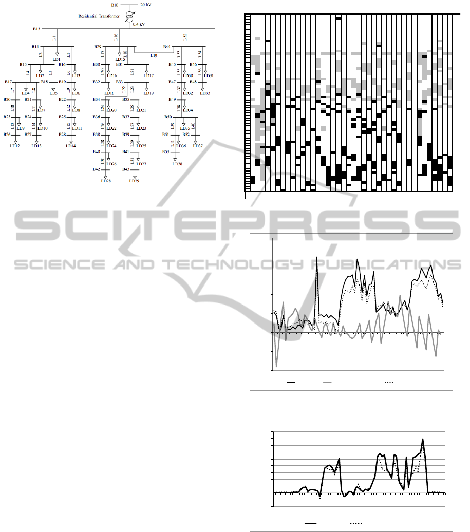
Figure 6. Topology of the low voltage residential grid. B denotes busses, L denotes cables and LD denotes
aggregated loads.
Table 2. Transformer station parameters.
Level
Ratings
Resistance [𝛀]
Reactance [𝛀]
Number of
taps
Voltage per tap [%
of nominal
voltage]
MV T1
50 MVA,
60/20 kV
3
13
10
(on-load)
1.25
MV T2
50 MVA,
60/20 kV
3
13
10
(on-load)
1.25
LV
industry
1250 kVA,
20/0.4 kV
0.001
0.02
2
(off-load)
2.5
LV
agriculture
200 kVA,
20/0.4 kV
0.002
0.05
2
(off-load)
2.5
LV
commercial
400 kVA,
20/0.4 kV
0.004
0.04
2
(off-load)
2.5
LV
residential
400 kVA,
20/0.4 kV
0.004
0.04
10
(on-load)
1.25
Figure 5: Low voltage benchmark grid.
5.2 Simulation Results
The simulation of the controller operation shows that
we can schedule higher loads than in the current grid
in such a way, that the grid infrastructure needs not be
enhanced.
We associated one house per bus, in total 38
houses and started the simulation at 6 AM during the
month of January. Because of the lower number of
houses in the experiment, the voltage limits have been
tightened from 10% down to 5% around the nominal
voltage.
In Figure 6 we illustrate the distribution of the
loads on the buses: the black colored heating periods
(more than 5kW) are alternating among the house-
holds represented on the columns of the diagram. The
light grey regions correspond to loads between 1 and
4.9 kW and are mainly caused by EV charging. The
uncolored rest is background load. Heating is more
frequent in the evening (towards the bottom of the fig-
ure)
The overall system operation in energy closed
loop is illustrated in Figure 7, in which we plot the
sum of the bus loads and the sum of power setpoints
in the time from 6am to 12pm. We observe that loads
and setpoints follow each other. On the same axis are
shown the energy prices c
j
, relative to the base price
of 44,23 Euro/MW, and the effect of negative prices
on the consumption increase.
Considering a certain bus in detail, the load and
setpoint values converge as well. The load and set-
points of household LD2 are shown in Figure 8. EV
charging occurs from periods 12 to 28 and from 40 to
64). Heating takes place in period 28 and from 62 to
64. Note that the setpoint that is limited by the voltage
and current limits is only partially followed by actual
CEMS load.
!
Figure 6: Schedule of consumption load among the CEMS
during the simulation.
-40
-20
0
20
40
60
80
100
1 3 5 7 9 11 13 15 17 19 21 23 25 27 29 31 33 35 37 39 41 43 45 47 49 51 53 55 57 59 61 63 65 67 69 71
Power [kW]
relative price [€/MW]
Time periods
total load relative energy price total ref. power
Figure 7: Total load and total reference power (setpoint)
during the simulation. Prices are relative to the base price.
-2
-1
0
1
2
3
4
5
6
7
8
9
1 4 7 10 13 16 19 22 25 28 31 34 37 40 43 46 49 52 55 58 61 64 67 70
Power&[kW]&
Time&periods&
Load at ld2 Setpoint at LD2
Figure 8: Load and setpoint at LD2 during the simulation.
In correlation with the setpoint (and the load) we
depict in Figure 9 the voltage evolution at LD38,
which is situated at the end of a feeder. The voltage
constraint in (19) V
min
= .95 is often hit during lunch
time and in the evening.
In a further series of simulations, we examine the
performance of the EV charging. Several factors have
SMARTGREENS2015-4thInternationalConferenceonSmartCitiesandGreenICTSystems
330

!"#$%
!"#&%
!"#'%
!"#(%
!"#)%
!"#*%
!"#+%
!"##%
,%
,"!,%
-./01
23%
Voltage
3.4%-10543%62&+%
7$%
!%
$%
'%
)%
,% &% (% *% #% ,,%,&%,(%,*%,#%$,%$&%$(%$*%$#%&,%&&%&(%&*%&#%',%'&%'(%'*%'#%(,%(&%((%(*%(#%),%)&%)(%)*%)#%*,%
Load%
Figure 9: Setpoint and voltage at the household LD38 dur-
ing the simulation.
18.00
18.20
18.40
18.60
18.80
19.00
19.20
19.40
19.60
1 4 7 10 13 16 19 22 25 28 31 34 37 40 43 46 49 52 55 58 61 64 67 70
°Celsius
Time periods
PV#on# PV#off#
Figure 10: Comparison of average inside temperature dur-
ing the simulation with and without PV.
an impact, such as the local generated power from PV
and the energy price, both a function of the charging
time of day.
The local generation does not appear in the power
flows in the grid, but has an impact on the inside house
temperature and on the energy stored in the batteries.
Figure 10 compares the inside temperature, aver-
aged over the houses: if PVs are on, the temperature
increases during the sunny hours. The same effect is
observed with the charged energy E
EV
, in Table 2. In
general (during sunny hours) the PV generation adds
energy to the battery (not much because of the low PV
generation in winter).
Table 2: Comparison of EV charged energy in percent from
D
max
during the day hours, with and without PV, (** in
[kWh], * in % of D
max
).
BUS EV parking E
EV
* E
EV
* D
min
D
max
noPV PV * **
LD1 8am-12am 19 21.3 19 8.8
LD2 4pm-7pm 55 55 47 11.6
LD3 1pm-11pm 67 62 45 8.6
LD5 3pm-6pm 45.6 45.6 45.6 8.0
LD13 11am-4pm 37 43 37 6.8
LD30 9am-3pm 60.5 73 60.5 7.2
LD32 4pm-8pm 78 78 78 5.9
LD33 11am-4pm 45 47 45 8.4
LD34 6pm-9pm 22 22 22 6.8
5.3 Discussion
The described system is complex as it includes sev-
eral load models and a lot of constraints that stabilize
its operation, such as energy prices, limitation of cur-
rents and voltages, flexibility limits, to consider only
a part. For the sake of a comparison, we assume that
prices have no influence and that the aggregation con-
troller provides each household with the energy it asks
for. Note that, even in this particular case, a six hours
load plan exists both at the aggregator and the CEMS
side, and that correct heating and charging function-
ality are not affected. One evaluation criterium is the
power quality, e.g. the frequency of the under-voltage
occurances, in our case voltages under 95% of the
nominal value. The simulation creates peak loads as
expected, such that 8.4% of the voltage measurements
are below the limit, compared to zero occurances, if
the aformentioned constraints were active, see Figure
11.
0"
10"
20"
30"
40"
50"
60"
70"
80"
90"
100"
0.84" 0.85" 0.86" 0.87" 0.88" 0.89" 0.9" 0.91" 0.92" 0.93" 0.94" 0.95"
under&voltage-
occurances-
Voltage-[pU]-
Figure 11: Simulation without price information and with-
out voltage limit checks. Histogram of under-voltage occu-
rances.
6 CONCLUDING REMARKS AND
FURTHER RESEARCH
In this work we address the energy management of
distributed energy resources using power and energy
flexibility information. In the selected residential sce-
nario, we define two interconnected controller enti-
ties, the CEMS controller and the aggregated energy
controller, and the appropriate energy optimization
models. The approach is based on forward planning
and optimized scheduling. Load predictive models
are crucial for the demand side management mech-
anism presented. Day ahead prices are used to penal-
ize or encourage demand at certain times of the day.
Eventual congestion is avoided by limiting the power
flows (voltages and currents). If we relax the condi-
tions above, the power quality deteriorates drastically.
In an experiment with a moderately loaded grid we
UsingFlexibilityInformationforEnergyDemandOptimizationintheLowVoltageGrid
331

obtained 8.4% under voltage events from a total num-
ber of 3024 voltage measurements in the whole LV
grid.
The benefit of using the flexibility information to
control the assets is difficult to quantify in normal
operation conditions: the EVs are charged to the re-
quired amount and the temperature is the houses re-
mains within limits. We think that the real benefits
of this architecture will be better visible in real world
and failure cases, to be studied in the future:
• errors in the prediction of charging activities pa-
rameters such as plugin and leaving time, demand,
of heating requirements, of non-flexible load, of
the solar irradiation, etc.
• failure through the temporary disconnection of the
communication network between the controllers,
or failure of the metering data collection. Normal
operation of loads and generators would continue
for longer time in our proposed system than in a
system without flexibility information exchange.
Finally, in this work it has been assumed that the
aggregated energy management is done by the DSO,
with input from the market actors (prices, available
energy, etc.). However, if this functionality is imple-
mented by a third party as part of a demand response
system, then the grid topology information might not
be available at the third party. In such a case a future
system architecture should provide better interactions
between DSO and market actors, and in the same time
it should provide cooperative decisions vis-a-vis the
consumers, similarly to the joint optimization prob-
lem solved by the aggregator.
ACKNOWLEDGEMENTS
The research leading to these results has received
funding from the European Communitys Seventh
Framework Programme (FP7/2007-2013) under grant
agreement no 318023 for the SmartC2Net project.
REFERENCES
Biegel, B., Andersen, P., Stoustrup, J., Hansen, L. H.,
and Tackie, D. V. (2013, June). Information model-
ing for direct control of distributed energy resources.
In American Control Conference (ACC), 2013 (pp.
3498-3504). IEEE.
Sundstrom, O.; Binding, C., ”Flexible Charging Optimiza-
tion for Electric Vehicles Considering Distribution
Grid Constraints,” IEEE Transactions on Smart Grid,
vol.3, no.1, pp.26,37, March 2012.
Lopes, J. A. P., Soares, F. J., and Almeida, P. M. R. (2011).
Integration of electric vehicles in the electric power
system. Proceedings of the IEEE, 99(1), 168-183.
CEN-CENELEC-ETSI Smart Grid Coordination
Group, Smart Grid Reference Architecture.
http://ec.europa.eu/energy/gas electricity/ smart-
grids/doc/xpert group1 reference architecture.pdf,
2012.
Harbo, S., and Biegel, B. (2013, October). Contracting flex-
ibility services. In Innovative Smart Grid Technolo-
gies Europe (ISGT EUROPE), 2013 4th IEEE/PES
(pp. 1-5). IEEE.
R. Pedersen, C. Sloth, G. B. Andresen, and R. Wisniewski,
DiSC - A Simulation Framework for Distribution Sys-
tem Voltage Control, 2014.
Andersson, G. (2012). Dynamics and control of electric
power systems. Lecture notes, 227-0528.
Binding, C., Dykeman, D., Ender, N., Gantenbein, D.,
Mueller, F., Rumsch, W. C., ... and Tschopp, H. (2013,
November). FlexLast: An IT-centric solution for bal-
ancing the electric power grid. In Industrial Electron-
ics Society, IECON 2013-39th Annual Conference of
the IEEE (pp. 4751-4755). IEEE.
Molderink, A., Bakker, V., Bosman, M. G., Hurink, J. L.,
& Smit, G. J. (2010). Management and control of do-
mestic smart grid technology. IEEE Transactions on
Smart Grid, 1(2), 109-119.
Orda, L. D., Bach, J., Pedersen, A. B., Poulsen, B., &
Hansen, L. H. (2013, October). Utilizing a flexibil-
ity interface for distributed energy resources through
a cloud-based service. In Smart Grid Communications
(SmartGridComm), 2013 IEEE International Confer-
ence on (pp. 312-317). IEEE.
Tu
˘
sar, T., Dovgan, E., & Filipic, B. Scheduling of flexible
electricity production and consumption in a future en-
ergy data management system: problem formulation.
In Proceedings of the 14th International Multiconfer-
ence Information SocietyIS 2011 (pp. 96-99).
Palensky, P., and Dietrich, D. (2011). Demand side manage-
ment: Demand response, intelligent energy systems,
and smart loads. Industrial Informatics, IEEE Trans-
actions on, 7(3), 381-388.
SmartC2Net official webpage, online: http://
www.SmartC2Net.eu.
Gurobi Solver webpage, online: www.gurobi.com
AMPL language webpage, online: www.ampl.com
SMARTGREENS2015-4thInternationalConferenceonSmartCitiesandGreenICTSystems
332
