
On Modeling the Cardiovascular System and
Predicting the Human Heart Rate under Strain
Melanie Ludwig, Ashok Meenakshi Sundaram, Matthias F¨uller,
Alexander Asteroth and Erwin Prassler
Bonn-Rhein-Sieg Univ. of Applied Sciences, Grantham-Allee 20, 53757 Sankt Augustin, Germany
Keywords:
Modeling and Predicting Behavior of Cardiovascular System, Adaptive Generation of Training Plans,
Automated Generation of Training Plans, Model-predictive Control of Smart Training Devices.
Abstract:
With the increasing average age of the population in many developed countries, afflictions like cardiovascular
diseases have also increased. Exercising has a proven therapeutic effect on the cardiovascular system and can
counteract this development. To avoid overstrain, determining an optimal training dose is crucial. In previous
research, heart rate has been shown to be a good measure for cardiovascular behavior. Hence, prediction of the
heart rate from work load information is an essential part in models used for training control. Most heart-rate-
based models are described in the context of specific scenarios, and have been evaluated on unique datasets
only. In this paper, we conduct a joint evaluation of existing approaches to model the cardiovascular system
under a certain strain, and compare their predictive performance. For this purpose, we investigated some
analytical models as well as some machine learning approaches in two scenarios: prediction over a certain
time horizon into the future, and estimation of the relation between work load and heart rate over a whole
training session.
1 INTRODUCTION
Many developed countries today face a global phe-
nomenon with dramatic consequences: the over-aging
of their societies. According to a WHO report (WHO,
2012) the average life expectancy in Europe has in-
creased by not less than five years between 1980 and
2010. While this seems to be good news in the first
place, the bad news follow instantly: with the demo-
graphic change, also the frequency of so-called so-
cietal diseases has increased dramatically. Europe
spends more than 500 bn Euro
1
per year to deal with
the effects of cardiovascular diseases, diabetes, high-
blood pressure, arthrosis, obesity just to name some
of them. Further to that cardiovascular diseases are
the main causes of death with almost 50% in western
industrial nations (Graf et al., 2014).
1
This figure is extrapolated from the cost incurred in Ger-
many by burn-out, cardiovascular diseases, and obesity
only, which in 2010 totaled to approx. 103 bn EUR. It
does not include other major cost driver such as athrosis
or dementia. In Europe the cost incurred by cardiovascu-
lar diseases only amounted to 195 bn EUR (Nichols et al.,
2012) in 2012.
One medication for most, if not all of these dis-
eases is exercising: walking, running, swimming, bik-
ing, hiking. But like for any medication it is the dose
that matters. Too much and wrong exercising can do
more harm to one’s health than it might use. Any
physical mobilization and training activity for a hu-
man subject therefore must be highly sensitive with
respect to the subject’s physical capabilities and ac-
tual physical condition in order to be effective. Ignor-
ing the limits of the physical capabilities will come
with a high risk of overstraining the subject and will
not only nullify the effect of the exercise but also re-
duce the motivation of the subject.
In order to avoid overstraining of the subject the
trainer or therapist that plans the workout must have
the ability to understand and predict with reasonable
accuracy how the subject’s cardiovascular system will
respond to a certain exercise strain. An easy to mea-
sure response index of the cardiovascular system is
the heart rate (HR), which is used in many mobile
applications and training devices to monitor the sub-
ject’s exercise. What is needed for a reliable predic-
tion is a model that establishes a functional relation
between the strain to which the subject is exposed and
106
Ludwig M., Meenakshi Sundaram A., Füller M., Asteroth A. and Prassler E..
On Modeling the Cardiovascular System and Predicting the Human Heart Rate under Strain.
DOI: 10.5220/0005449001060117
In Proceedings of the 1st International Conference on Information and Communication Technologies for Ageing Well and e-Health (ICT4AgeingWell-
2015), pages 106-117
ISBN: 978-989-758-102-1
Copyright
c
2015 SCITEPRESS (Science and Technology Publications, Lda.)

the response of the cardiovascular system.
The purpose of the work described in this paper is
to evaluate which approaches to model the heart rate
dynamics for moderate exercises exist today in gen-
eral and which prediction performance they show in
particular. This prediction performance is crucial in
two respects: First it will guide the elaboration of ex-
ercises for a subject as already indicated above. Sec-
ond an accurate prediction of the response of the heart
rate to a certain strain will be essential to control smart
training devices such as treadmills, elliptical trainers
in indoor environments or Pedelecs or mobile apps in
outdoor environments to control the strain which they
impose on a subject. Only if these devices and their
respective control systems incorporate models with a
decent predictive performance will they be able to de-
termine the right dosing of strain that leads to an op-
timal training or therapy result.
We divided the existing approaches to modeling
the heart rate response to running exercise into two
classes: a) analytical models, whose parameters need
to be identified based on some given data sets, and
b) machine learning approaches, which try to learn
and generalize the stimulus response patterns with-
out a prior model. While the first class of approaches
gains its appeal from its analytical close-form nota-
tion, the second class is attractive because it also al-
lows accounting for environmental parameters such
as altitude, slope, or any other relevant information.
Representatives of both classes are described below.
The description is followed by a comprehensive eval-
uation of the prediction performance of the respective
approaches.
2 STATE OF THE ART
Fitness devices such as GPS watches, step coun-
ters, or smartphones apps
2
are widely applied for car-
dio sports. These devices monitor a person’s heart rate
and issue an alarm if the heart rate is above or below a
given threshold. They do not influence the exercise di-
rectly, i.e. by providing some haptic feedback. Most
of these apps and devices are connected to web por-
tals that provide a visualization of a subject’s training
data and recommend certain exercises. However, the
recommendations are rather minimalistic and include
only the duration of an exercise and set-point values
for the heart rate. Detailed training plans are typi-
cally only provided by human experts but not gener-
ated automatically from recorded data. The subjects
have to control their heart rates themselves based on
2
e.g. http://www.garmin.com, http://www.polar.com,
http://www.runtastic.com
their experience. To improve the automated genera-
tion of training plans and control a subject’s perfor-
mance correctly, the response of the subject to certain
exercise strain needs to be modeled.
Models that describe a subject’s response to a
workload have been studied for decades (Calvert
et al., 1976; Hajek et al., 1980). The most common
applications for these models are control systems for
treadmills or ergometers. A well-known model for
these types of control systems has been presented by
(Cheng et al., 2007; Cheng et al., 2008). These au-
thors introduce a nonlinear state-space model to pre-
dict the heart rate behavior of a subject based on the
running velocity on a treadmill. This model includes
nonlinear components to simulate changes in the or-
ganism due to long term exercises. (Paradiso et al.,
2013) use the same model to regulate the heart rate us-
ing a cyclic ergometer. They further show the generic
application of this model to different sports activities.
(Baig et al., 2010) uses a second order LTI model to
describe the response for cycling, walking and rowing
exercises. Their model uses the exercise frequency as
input. (Mohammad et al., 2011) uses a Hammerstein
model for cycling exercises on a home trainer. Similar
model-based systems for running or cycling or row-
ing on different training devices can be found in (Su
et al., 2007; Koenig et al., 2009; Zhang, 2013; Leitner
et al., 2014). With the use of smartphones and their
sensors, new response model applications have been
investigated. (Velikic et al., 2011) uses accelerome-
ter information to predict the heart rate for a specific
activity up to one hour. (Sumida et al., 2013) esti-
mates the heart rate dynamics via smart phone sensor
data that are analyzed by a neural network. The en-
vironmental condition is included as a gradient factor
as well. However, the proposed model is so far only
tested for walking and hiking.
In the recent past, the use of machine learning
techniques to model the nonlinear relation between
the heart rate and its affecting factors has gained some
attention. Support vector regression is used in (Wang
et al., 2009) to study the nonlinear behavior of cardio-
vascular variables. This resulted in a nonparametric
model that quantitatively describes the observations
made. In (Javed et al., 2009) the relation between
blood volume and heart rate is modeled. The parame-
ters for support vector regression were selected based
on grid search approach combined with k-fold cross
validation. It uses radial basis function among many
other available nonlinear kernels. Evolutionary neural
networks were used to predict the heart rate in (Feng
Xiao et al., 2010). Neural networks are highly ca-
pable in modeling nonlinear pattern in the data. But
the structure and weights of net plays a important role
OnModelingtheCardiovascularSystemandPredictingtheHumanHeartRateunderStrain
107
in this. Using evolutionary techniques to find the best
structure and weight of the nets in the available search
space ensures this. Heart rate variability is modeled as
linear combinations of Gaussians mixtures in (Costa
et al., 2012).
Beside the usage in a control system, models of
the cardiovascular system can also be used for auto-
mated training plan generation. (Brzostowski et al.,
2013) presents an eHealth application that uses an an-
alytical model as described in (Cheng et al., 2007) in
order to generate an optimal training protocol to avoid
overstrain. The training protocol includes only esti-
mated running speed and does not include environ-
mental conditions. (M¨uller et al., 2014) evaluated the
generic heart rate model that is capable of transferring
the response of a subject between cycling and running
exercises. They include their model in a training plan
generation system that is capable of predicting the re-
sponse of a certain training in advance.
The presented literature provides solutions to esti-
mating the heart rate based on some specific exercise
strain. However, the results are not comparable since
all of them have used different types of exercises and
workloads. One comparison of mathematical models
can be found in (Lefever et al., 2014). They com-
pared different time-variant mathematical models for
outdoor cyclic trainings. The study presented here is
a first step towards the evaluation of analytical mod-
els and machine learning techniques for running exer-
cises.
3 MODELING AND PREDICTION
3.1 Experimental Setup and Data
Generation
The experimental data for the analysis and system
identification were recorded for a 27 years old fe-
male subject on a treadmill with a constant gradient of
1.5% and different velocities based on different exer-
cise protocols. Every protocol starts with a three min-
utes resting phase to record the resting heart rate of
the subject. To cover different aspects for the model
identification, three types of exercises were used:
• The first was a simple onset-offset exercise. The
subject ran for 15 minutes with a constant speed
of 8km/h .
• The second was a step exercise protocol. It started
with 7km/h and increased the speed by 2km/h ev-
ery six minutes. The exercise stopped after a ve-
locity of 13km/h was reached.
• The third type of exercise was an interval proto-
col with two alternating velocities. The exercise
started with 12 km/h for seven minutes, followed
by a resting phase of 8km/h for five minutes, in-
creased again to 12km/h for seven minutes and
finished with a 8km/h phase for five minutes.
0 500 1000 1500 2000
50
100
150
200
time (s)
heart rate (bpm)
0 500 1000 1500 2000
−10
0
10
20
velocity (km/h)
measured heart rate
velocity
Figure 1: Example data set for exercise type 3 (interval).
In our experiments we recorded the following perfor-
mance data: time in seconds (s), distance in kilome-
ters (km), velocity in kilometers per hour (km/h), al-
titude in meter (m), and heart rate in beats per minute
(bpm). These data were sampled by our measurement
setup in 10 seconds intervals and added to the data set
throughout the entire session. All exercises were fol-
lowed by a five minute resting phase to measure the
recovery capabilities of the heart rate. Figure 1 shows
an example data set of exercise type three. All in
all, five exercises of each type have been performed,
resulting in a complete set of 15 recorded sessions.
These sessions have been used in the following model
identification and learning process.
3.2 Modeling Approaches
As pointed out earlier, these modeling approaches can
be divided into two classes: (i) the class of analyt-
ical models, whose parameters have to be identified
based on a set of training data, and (ii) the class of
machine learning approaches, which do not refer to
a prior model but learn a model that fits the training
data during a learning phase.
3.2.1 Analytical Models
In all analytical models and experiments, velocity im-
posed on the subject (the runner) as workload and is
hence considered as input parameter u. The output
is a prediction of the heart rate that is associated with
ICT4AgeingWell2015-InternationalConferenceonInformationandCommunicationTechnologiesforAgeingWelland
e-Health
108

this workload through the respective analytical model.
Each model is made up of a specific number of param-
eters, which can be used for adapting the model to the
subject. First, we would shortly describe each model
and illustrate the used method for parameter identifi-
cation afterwards.
• Cheng ODE Model (Cheng et al., 2007): The dif-
ferential equation model from Cheng et al. is orig-
inally used for treadmill walking and is described
as follows:
˙x
1
= −a
1
x
1
(t) + x
2
(t) + g(u(t))
˙x
2
= −a
4
(x
2
(t) − tanh(x
2
(t))) + a
5
x
1
(t)
y(t) = x
1
(t)
with g(u(t)) =
a
2
u
2
(t)
1+exp(−u(t)+a
3
)
and initialization
x(0) = [x
1
(0) x
2
(0)]
′
= [0 0]
′
. Additional
points in time are set to zero. Changes in heart
rate were modeled by x
1
, whereas x
2
represents
the reaction of human metabolism in dependency
of x
1
like effects from hormonal system, increase
in body temperature or other slow-acting effects.
The output y(t) = ∆HR(t) = HR(t) − HR
rest
de-
scribes the changes in heart rate from resting heart
rate. The model uses five parameters a
1
, ..., a
5
∈
R
+
.
• Paradiso ODE Model (Paradiso et al., 2013):
The differential equation model from Paradiso et
al. is used for cycling. The second-order time-
invariant nonlinear system is described as
˙x
1
(t) = −a
1
x
1
(t) + a
2
x
2
(t) + a
6
u
2
(t)
˙x
2
(t) = −a
3
x
2
(t) + a
4
f
a
5
(x
1
(t))
where f
a
5
is a Lipschitz continuous function
in dependency of a
5
like f
a
5
(x
1
(t)) = x
1
(t) ·
1
1+e
−x
1
(t)−a
5
. The output x
1
(t) = ∆HR(t) describes
the changes in heart rate from resting heart rate
and x
2
models the slow-acting effects similar to
the model from (Cheng et al., 2008). The model
uses six parameters a
1
, ..., a
6
∈ R
+
.
• LTI Model (Baig et al., 2010): The second order
linear time invariant model as below is used for
heart rate prediction during walking, cycling and
rowing exercise:
y(t) = a
1
· y(t − 1) + a
2
· y(t − 2)
+ a
3
· u(t − 1) + a
4
· u(t − 2)
where y(t) = ∆HR(t) is the measured change in
heart rate at time t. The model uses four parame-
ters a
1
, ..., a
4
∈ R.
• Takagi-Sugeno Model (Mohammad et al., 2011):
This modified Hammerstein model is usually used
for elderly non trained people. Let x be an n-
element sequence with elements in R
3
and we
identify the first element of the first component
with the resting heart rate, zero else. Then it is:
x(t + 1) = (Ax)(t) +
2
∑
i=0
h
i
(u(t))B
i
u(t) + B
u0
with
h
1
(u(t)) =
u(t) − u
min
u
max
− u
min
, h
2
(u(t)) =
u
max
− u(t)
u
max
− u
min
,
and B
1
= B
u1
+ u
max
B
u2
, B
2
= B
u1
+ u
min
B
u2
and
A =
a
1
1 0
a
2
0 1
a
3
0 0
, B
ui
=
γ
0i
γ
1i
γ
2i
.
The sequence of the approximated heart rate y is
given by y(t) := x
1
(t). The model uses twelve pa-
rameters a
i
, γ
0i
, γ
1i
, γ
2i
∈ R, i ∈ {1, 2, 3}.
For all models, to identify the suitable model pa-
rameters, we used the workload data and the mea-
sured heart rate as input. We fitted the modeled heart
rate to actual measured heart rate by using a recur-
sive least square algorithm (Levenberg-Marquardt al-
gorithm) for minimizing the error like recommended
in (Busso et al., 1997). Therefore, we made a leave-
one-out cross validation where we used 14 data sets
to simultaneously identify the parameter setting for a
model and used these parameters in evaluation for the
remaining one data set.
3.2.2 Machine Learning Approaches
In the following paragraphs, we describe three ma-
chine learning approaches to modeling and predicting
the heart rate of a subject during an exercise. The in-
put for the three learning approaches consists of nine
features. Three of them describe the current work-
load: the running velocity, distance run and the run-
ning altitude. The six remaining input features consist
of the six subsequent samples of the heart rate that im-
mediately precede the time of prediction. Our heart
rate monitor yields a new sample every ten seconds.
This means that six subsequent samples correspond to
a time horizon of sixty seconds in the exercise and the
data set respectively.
The idea to refer to a sequence of preceding heart
rate samples for modeling the response of the heart
to strain was discussed already in (Feng Xiao et al.,
2010). Not surprisingly we find a nearly linear rela-
tion between the current sample of the heart rate and
a short sequence of heart rate samples immediately
preceding the current sample. Figure 2 shows the cor-
relation between the previous instances of the heart
OnModelingtheCardiovascularSystemandPredictingtheHumanHeartRateunderStrain
109

rate to the current heart rate in the dataset. As a trade
off between the correlation pattern and also in order
to avoid unnecessary high dimension, we chose only
six previous instances as features. As a preprocessing
step in all approaches, we standardize the data to have
zero mean and unit variance.
0.55
0.6
0.65
0.7
0.75
0.8
0.85
0.9
0.95
1
hr(t−1) hr(t−2) hr(t−3) hr(t−4) hr(t−5) hr(t−6)
Previous HR samples
Correlation Coefficient
MSE: long term prediction
Figure 2: Correlation of current heart rate sample with pre-
vious heart rate samples.
• Linear Regression (LR) (Seal, 1967) is a statisti-
cal technique used to model the relation between
input explanatory variables and output response
variables by using a linear predictor function. The
model is a linear combination of explanatory vari-
ables as described below.
ˆy(w, x) = w
0
+ w
1
x
1
+ ... + w
p
x
p
ˆy is the response variable, x = (x
1
, ..., x
p
) are the
explanatory variables, p is the number of explana-
tory variables, w = (w
1
, ..., w
p
) are the unknown
coefficients and w
0
is the intercept. The unknown
coefficients and intercept are identified using the
least square algorithm to minimize the residual
sum of squares between the observed and pre-
dicted responses. A reliable model requires a sig-
nificant correlation between the explanatory and
response variables. Detailed formulation on this
regression approach can be found, for example, in
(Tabachnick and Fidell, 2006). For training and
testing the heart rate prediction, the nine features
described earlier will act as the explanatory vari-
ables and the heart rate is the response variable.
Linear regression is also studied for heart rate re-
sponse in (Javed et al., 2009).
• Multilayer Perceptron (MLP) (Rosenblatt,
1961) is a feedforward type artificial neural
network used to map input values to the corre-
sponding outputs. The basic structure of a MLP
include an input layer, a number of hidden layers
followed by an output layer. The nodes in each
layer are fully connected to the nodes in the
subsequent layer. The nodes in hidden layers
and output layer additionally have an activation
function which is linear or nonlinear depending
on the application. In our application the network
has three hidden layers with sigmoid activation
functions. The weights of the links that connect
the nodes in each layer are usually learned by
supervised learning techniques using the given
training data. We use the back propagation
technique along with gradient descent to learn the
weights. Mathematically, each non-input layer
in the network can be described by the following
equation:
y = ϕ(w
T
x+ b)
where y is the output to next layer, x is the in-
put vector from the previous one, w is the weight
vector, b is the bias and ϕ is the activation func-
tion. The training data is provided multiple times
known as epochs in order to avoid local minima to
a certain extent. For training and testing the heart
rate prediction, the nine features described earlier
act as the input and the predicted heart rate is the
output. It takes the network about 500 training
epochs with 20% cross validation set to approxi-
mate the true output value with a decent accuracy.
Neural networks for heart rate prediction are also
discussed in (Feng Xiao et al., 2010) and (Sumida
et al., 2013).
• Support Vector Regression (SVR) introduced by
(Vapnik, 1995) is based on Vapnik-Chervoenkis
theory. If {(x
1
, y
1
)...(x
n
, y
n
)} ⊂ χ × R is a given
training data where χ is the input space, the goal
is to find a function f (x) = w · φ(x) + b that has
at most ε deviation from actual targets and at the
same time remain as flat as possible. φ(x) is
in a high-dimensional space which is nonlinearly
transformed from x by using an appropriate ker-
nel which in our case is radial basis function. The
coefficients w and b are identified by minimizing
a regularized risk function while considering the
allowed ε deviation. The regularization constant
and ε can be varied and defined by the subject.
Improper selection of these values could result in
over or under fitting of the data. A grid search
over a possible combination of values combined
with k-fold cross validation technique is used to
identify the best one with minimal average mean
squared error. A detailed tutorial on SVR can be
found in (Smola and Sch¨olkopf, 2004). For train-
ing and testing the heart rate prediction perfor-
mance, the nine features described earlier act as
ICT4AgeingWell2015-InternationalConferenceonInformationandCommunicationTechnologiesforAgeingWelland
e-Health
110

the input variables and the heart rate is the out-
put variable. Use of SVR for cardiovascular sys-
tems can also be found in (Wang et al., 2009) and
(Javed et al., 2009).
3.2.3 Baseline Models
To mark a bottom line for the performance of our
modeling approaches we introduce what is called
baseline models. These models are very simple and
do not bear any physiological meaning. We expect
that all studied modeling approaches better explain
the processes underlying the data sets and hence more
accurately fit the datasets than these baseline models.
We use a polynomial model as baseline for the predic-
tion of an entire session and a simple point shift model
as baseline for the prediction over different time hori-
zons. Note that due to noise and other effects a model
that tries to explain a physiological causality is not
guaranteed to perform better than a baseline model.
• Polynomial Model: The modeled heart rate is
given by y(t) = a
0
+a
1
·u(t)+a
2
·u
2
(t) with three
parameters a
0
, a
1
, a
2
∈ R and velocity u. This
model is just a scaling function as easy as possi-
ble for mapping any kind of input data (like work-
load) to any kind of output data (like heart rate).
We used this function as baseline function to de-
termine the fitting-quality without any physiolog-
ical modeling.
• Pointshift Model: The modeled heart rate is pro-
duced as the measured heart rate with a time shift
according to the defined time horizon. To predict
w seconds, we call w the winsize and model the
heart rate y at each point of time t as y(t + w) =
hr(t) where hr is the measured or controlled heart
rate. The model stops when the training is fin-
ished. Any kind of workload is completely ig-
nored in this case.
3.3 Evaluation of Prediction
Performance
It the following section the approaches discussed in
the previous section are evaluated based on their pre-
diction performance measured as mean squared errors
(MSE). Throughout this evaluation, out of a total of
15 data sets, 14 were used for training and the re-
maining one was used for testing. This was repeated
combinatorially to have every data set used as a test
set at least once. So, in total, 15 experiments (cross
validations) were conducted for each evaluation.
3.3.1 Multi-step Prediction
In multi-step prediction, we are interested in pre-
dicting the heart rate over a certain time horizon
based on the current input data. Multi-step prediction
is needed, for example, to properly control the
strain that a smart training device imposes on a
subject during exercising. If the heart rate increases
or decreases unexpectedly, we need to reduce or
increase the workload on the subject in time. To do
this properly we need to predict how the heart rate
is going to evolve in the future depending on some
given input. The time horizons (w), over which the
prediction performance was evaluated, were 10, 20,
30, 60, 90, and 120 seconds. The polynomial model
by nature does not allow modeling and predicting the
heart rate over a longer time interval. Therefore we
use the pointshift model as baseline.
Prediction Performance of Analytical Models:
For the ODE as well as for the Takagi-Sugeno
model, we simulate the system up to time t while up-
dating the heart beat state with the current measure-
ments. From time t to t + w, we simulate the system
without any update. If we use the LTI model for heart
rate prediction with different time horizons like de-
scribed above, the parameter identification has to be
redone and adjusted to consider longer time horizons.
For predicting the next w seconds we have to take all
horizon sizes between 1 and w into account. The LTI
model was used for single step heart rate prediction in
(Baig et al., 2010). In this case, the average MSE is
about 6.7 bpm
2
.
The left part of table 1 shows the average MSE
(in bpm
2
) of the analytical models over all 15 test
sessions for different time horizons. As we can see,
the LTI model predicts better than the complex ODE
models as well as the respective baseline model for
each horizon size, but the deviation between the real
heart rate and the predicted heart rate gets worse for
longer time horizons. The performance of the Takagi-
Sugeno model is worse for small horizons compared
to a simple pointshift. However, it improves for big-
ger prediction horizons and is the best analytical ap-
proach for 120s horizons and above.
In Figure 3, the test set prediction performance
for a 60 seconds time horizon is shown as an example
for one training session. The upper figure shows the
prediction performance of the LTI model and the
lower figure shows the performance of the respective
baseline method. Apparently, the LTI model scales
the given velocity with an additional shifting to the
heart rate level without systematically overestimating
OnModelingtheCardiovascularSystemandPredictingtheHumanHeartRateunderStrain
111
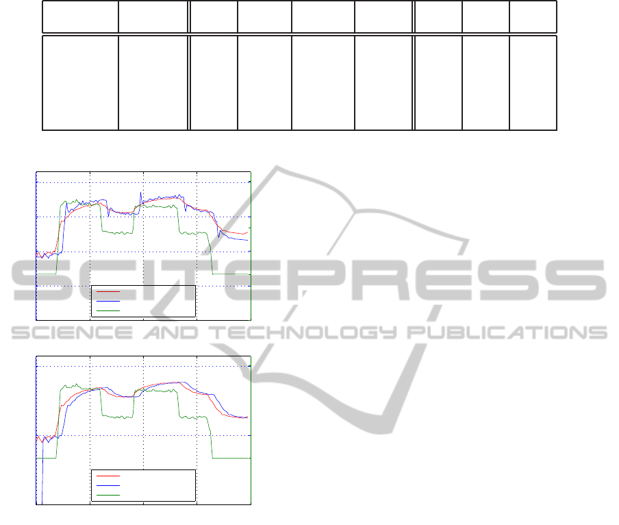
Table 1: Test set average MSE (in bpm
2
) of analytical and learning models for multi-step prediction.
prediction Cheng Paradiso Takagi-
horizon (s) Pointshift LTI ODE ODE Sugeno LR MLP SVR
10 8.54 6.67 23.61 9.95 22.89 5.70 6.43 5.72
20 16.19 13.07 50.22 23.19 26.83 16.43 19.34 16.62
30 23.84 19.12 68.08 36.85 34.98 24.09 28.92 24.60
60 48.51 37.61 98.05 68.84 50.79 37.93 50.16 39.92
90 76.60 59.23 114.84 93.54 57.02 44.92 64.39 48.44
120 108.64 85.99 133.34 123.25 65.31 50.13 76.34 55.73
0 500 1000 1500 2000
50
100
150
200
Model: Linear Time Invariant, Prediction
time (s)
heart rate (bpm)
0 500 1000 1500 2000
−10
0
10
20
velocity (km/h)
measured heart rate
predicted heart rate
velocity
0 500 1000 1500 2000
0
100
200
Model: Pointshift, Prediction
time (s)
heart rate (bpm)
0 500 1000 1500 2000
0
20
velocity (km/h)
measured heart rate
predicted heart rate
velocity
Figure 3: Example multi-step prediction for the LTI model
(upper figure: MSE = 30.75 bpm
2
) and the pointshift model
(lower figure: MSE = 31.58 bpm
2
) with a time horizon of
60 seconds.
or underestimating the real heart rate. Also it can
be observed that after adapting to a new velocity
the simulated heart rate has a greater variance in the
first few seconds. This does not happen with the
Pointshift model as it does not use the velocity at all.
Prediction Performance of Learning Approaches:
The three presented learning approaches LR, MLP,
and SVR, which were designed for a single-step pre-
diction in the first place, are also capable of perform-
ing multi-step predictions. As a matter of fact we can
use the algorithms for single-step prediction with a
small rearrangement of the input values to perform
multi-step prediction.
All three learning approaches use a history of
the past six heart rate samples {hr
s
(t − 5), . . . , hr
s
(t)}
covering a time span of 60 seconds in addition to
the workload parameters velocity, distance, and alti-
tude to predict the heart rate hr
p
(t + 1). If we want
to use the same approaches to predict the heart rate
hr
p
(t + 2) for time t + 2, would apparently have to
shift the history by one time step and use {hr
s
(t −
4), . . . , hr
s
(t)}. Our learning algorithms, however, ex-
pect six heart rate samples and not five. A sample
hr
s
(t + 1), however, is not available. To fix this prob-
lem we add our prediction for time hr
p
(t + 1) to the
history. Altogether the algorithm uses then the his-
tory {hr
s
(t − 4), . . . , hr
s
(t), hr
p
(t + 1)} and the actual
workload parameters, distance, velocity and altitude
at time t + 1 to predict the heart rate hr
p
(t + 2). If
we have to predict further into the future we would
update the history with our estimates hr
p
(t + 2).
Note that in principle this allows us to predict
the heart rate arbitrarily far into the future. Due to
the absence of any new samples of the heart rate,
which would give more insight into the true response
of the heart, we include more and more predictions
hr
p
(t + k) in our history. So the history will even-
tually be filled up with earlier predictions instead of
earlier true measurements. Naturally our predictions
will get worse and worse as we reach farther into the
future very much like a weather forecast.
The right part of table 1 shows the average MSE
over all 15 data sets for different time horizons. LR
predictions are comparatively better among the other
two for multi-step prediction. However, the perfor-
mance of SVR is also very close to that of LR.
In Figures 4, 5 and 6, the prediction performance
of LR, MLP and SVR with a 60 seconds time horizon
is shown as an example for one training session. With
a 60 seconds time horizon all three approaches seem
to predict fairly well. But the performance gets worse
as the time horizon size increases as explained earlier.
This is also due to the fact that all approaches
tightly depend on a history of sampled heart rates
rather than on other features. Future work shall ad-
dress a more comprehensive use of other features that
also contribute to the heart rate variation.
ICT4AgeingWell2015-InternationalConferenceonInformationandCommunicationTechnologiesforAgeingWelland
e-Health
112
0 500 1000 1500 2000
50
100
150
200
time (s)
heart rate (bpm)
Model: Linear Regression , Prediction
0 500 1000 1500 2000
−10
0
10
20
velocity (km/h)
measured heart rate
predicted heart rate
velocity
Figure 4: Example multi-step prediction for the LR model
with a time horizon of 60 seconds (MSE = 21.75 bpm
2
).
0 500 1000 1500 2000
50
100
150
200
time (s)
heart rate (bpm)
Model: Multilayer Perceptron , Prediction
0 500 1000 1500 2000
−10
0
10
20
velocity (km/h)
measured heart rate
predicted heart rate
velocity
Figure 5: Example multi-step prediction for the MLP model
with a time horizon of 60 seconds (MSE = 22.84 bpm
2
).
0 500 1000 1500 2000
50
100
150
200
time (s)
heart rate (bpm)
Model: Support Vector Regression , Prediction
0 500 1000 1500 2000
−10
0
10
20
velocity (km/h)
measured heart rate
predicted heart rate
velocity
Figure 6: Example multi-step prediction for the SVR model
with a time horizon of 60 seconds (MSE = 20.70 bpm
2
).
3.3.2 Session Prediction Performance
One main application of multi-step prediction is
the control of the strain imposed to a subject by
a smart training device. If instead the task is to
develop a sensitive training plan for a subject for a
whole workout session then a key question is if the
models – acquired either through parameter fitting
or through a learning approach – also describe the
input output relation between imposed strain and
resulting heart rate over a longer period of time. In
other words: For a given workload at a given time
will our models be able to yield a decent estimate
of the heart rate at that given point in time? We use
the term session prediction performance to refer to
this capability of our models
3
. We use the polyno-
mial model as a baseline model for session prediction.
Prediction Performance of Analytical Models:
50
100
150
200
250
300
350
400
Cheng Paradiso Takagi−Sugeno LTI Polynomial
MSE
Figure 7: Test set MSE (in bpm
2
) of analytical models for
session prediction.
The MSE for the analytical models over all test
data sets is shown in Figure 7. The Takagi-Sugeno
model has a much smaller variance in between the
25th and 75th percentiles as the other models and the
upper whisker is lower as well. Hence the prediction
quality is much higher for this model. In comparison,
the variance of the LTI model is quite similar to the
variance of the polynomial baseline model. It is worth
mentioning that all models have one outlier data set.
A closer look at these data shows that there is a
significant difference between the resting heart rate
in this one session compared to the common resting
heart rate in all other sessions. The resting heart rate
in this data set is approximately 20 bpm lower as in
the other sessions while the parameter setting is es-
timated on training sessions with the higher resting
heart rate exclusively. For the ODE models, the MSE
of this data set belongs to the upper whisker, for the
others it belongs to the outlier.
The average of the MSE is shown in the left part of
Table 2 for training as well as for testing. Especially
it can be seen that the test case for the Takagi-Sugeno
3
In estimation theory estimating the value of a function at a
given point in time based on the observations made up to
this point is denoted as filtering rather than predicting
OnModelingtheCardiovascularSystemandPredictingtheHumanHeartRateunderStrain
113
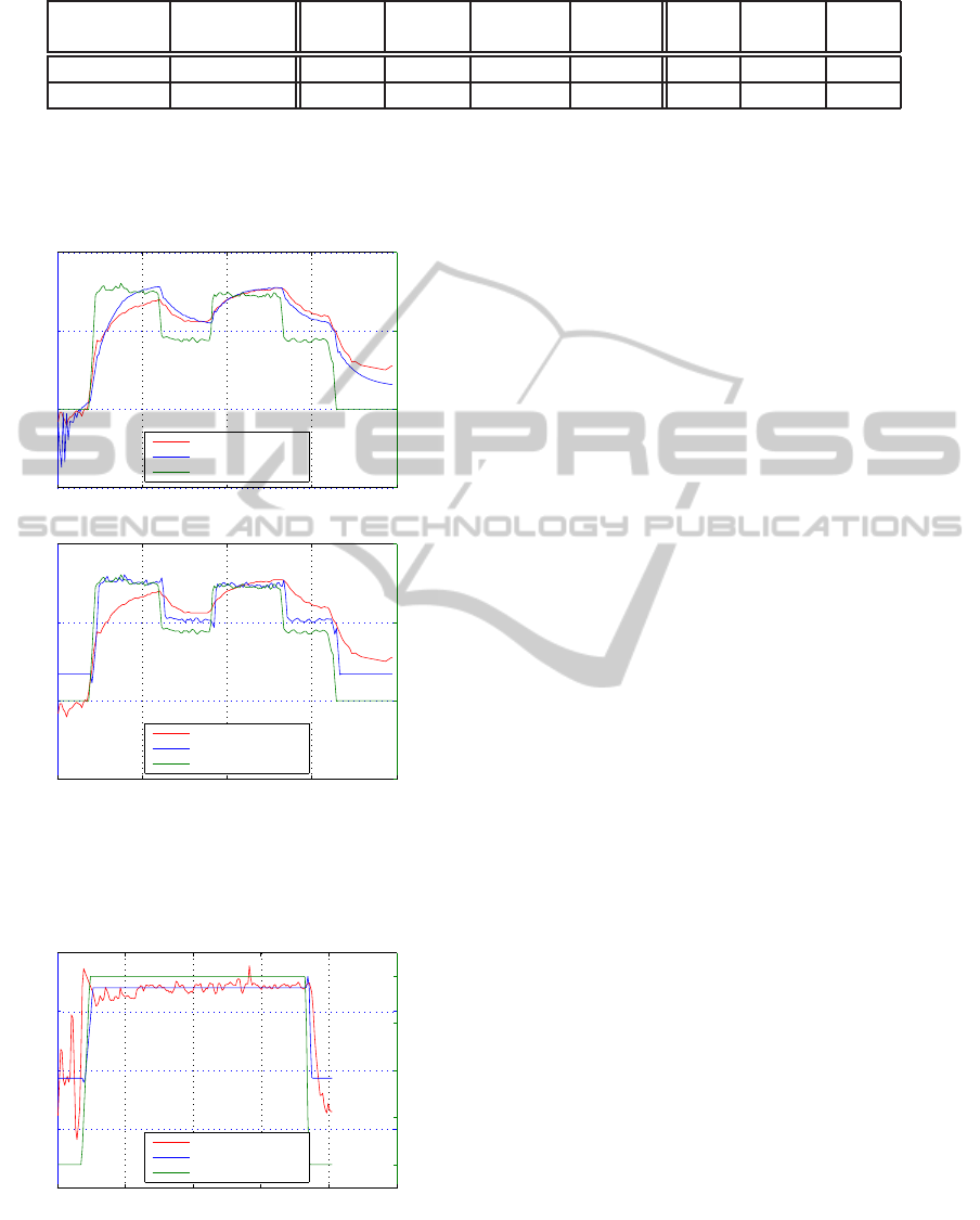
Table 2: Average MSE (in bpm
2
) of analytical and learning models for session prediction.
Cheng Paradiso Takagi-
Polynomial LTI ODE ODE Sugeno LR MLP SVR
training set 120.84 100.44 113.57 183.37 15.29 5.67 5.90 5.66
test set 159.70 131.24 124.75 191.17 74.70 66.28 124.48 79.40
model ended up with better results than the training
part for the LTI model and the baseline method.
0 500 1000 1500 2000
50
100
150
200
Model: Takagi−Sugeno, Prediction
time (s)
heart rate (bpm)
0 500 1000 1500 2000
−10
0
10
20
velocity (km/h)
measured heart rate
predicted heart rate
velocity
0 500 1000 1500 2000
50
100
150
200
Model: Linear Time Invariant, Prediction
time (s)
heart rate (bpm)
0 500 1000 1500 2000
−10
0
10
20
velocity (km/h)
measured heart rate
predicted heart rate
velocity
Figure 8: Example session prediction for the Takagi-
Sugeno model (upper figure: MSE = 41.27 bpm
2
) and the
LTI model (lower figure: MSE = 161.46 bpm
2
).
0 500 1000 1500 2000 2500
80
100
120
140
160
Model: Linear Time Invariant, Prediction
time (s)
heart rate (bpm)
0 500 1000 1500 2000 2500
0
2
4
6
8
velocity (km/h)
measured heart rate
predicted heart rate
velocity
Figure 9: Example session prediction for the LTI model
(MSE = 56.89 bpm
2
).
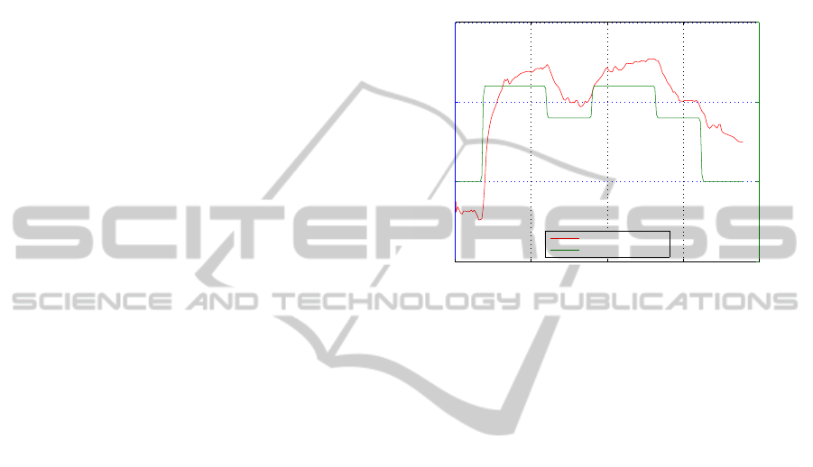
In Figure 8, the test set prediction performance
of Takagi-Sugeno model and LTI model are shown
for one exercise training session. In this case, the
MSE equals 41.27 bpm
2
for the Takagi-Sugeno model
and 161.46 bpm
2
for the LTI model. Furthermore,
the Takagi-Sugeno model overestimates the heart rate
after the first increase of velocity, but adapts quite
well after approximately 800 seconds. Even if the
time for better adaptation varies, the Takagi-Sugeno
model predicts better after the middle of the session
time compared to the beginning in most of our exper-
iments.
In comparison, the LTI model seems to be much
more dependent on the current velocity than on
the further measured heart rate. So there are huge
deviations between the measured heart rate and
the simulated one corresponding to an increase or
decrease of the velocity. This behavior is typical
for the LTI model in our experiments. Figure 9
provides an example of onset/offset training where
this behavior can be well used by the LTI model. The
MSE equals 56.89 bpm
2
in this case.
Prediction Performance of Learning Approaches:
In this section we evaluate the session prediction per-
formance of the three learning approaches: LR, MLP
and SVR. As stated earlier, we can use the models
initially learned/trained for a one-step prediction also
for a multi-step prediction, with a grain of salt that
the further we predict into the future the less accu-
rate our predictions will be. The key difference be-
tween multi-step prediction and session prediction is
the length of the time horizon. For session prediction
the complete session is considered as the time hori-
zon. Given that predictions into the far future become
more and more inaccurate this sounds like turning the
grain of salt into a rock of salt. Figure 10 shows that
the situation luckily is not as bad as one might think:
the LR algorithm for an entire session lasting about 35
minutes is on average about 8 bpm off the true value
with its prediction.
The mean squared error to predict all test data sets
is summarized in Figure 10. The average of these
mean squared errors for training and testing is shown
in Table 2. The prediction performance of all three
approaches for one example session is shown in Fig-
ure 11, 12 and 13.
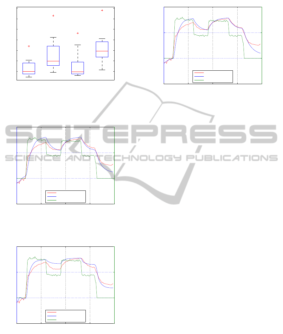
The session prediction performance apparently is
worse than multi-step prediction performance since
ICT4AgeingWell2015-InternationalConferenceonInformationandCommunicationTechnologiesforAgeingWelland
e-Health
114
50
100
150
200
250
300
350
LR MLP SVR Polynomial
MSE
Figure 10: Test set MSE (in bpm
2
) of learning approaches
for session prediction.
0 500 1000 1500 2000
50
100
150
200
time (s)
heart rate (bpm)
Model: Linear Regression, Prediction
0 500 1000 1500 2000
−10
0
10
20
velocity (km/h)
measured heart rate
predicted heart rate
velocity
Figure 11: Example session prediction for the LR model
(MSE = 43.30 bpm
2
).
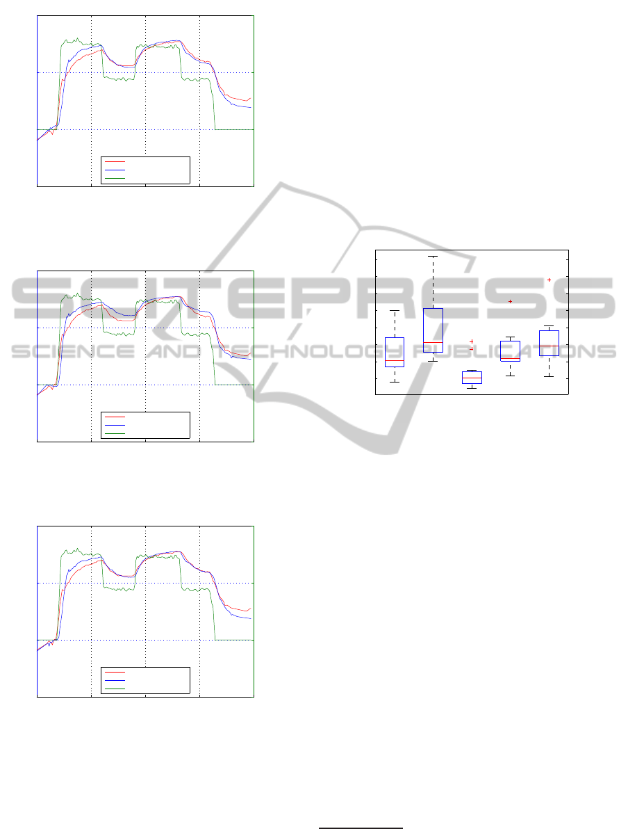
0 500 1000 1500 2000
50
100
150
200
time (s)
heart rate (bpm)
Model: Multilayer Perceptron , Prediction
0 500 1000 1500 2000
−10
0
10
20
velocity (km/h)
measured heart rate
predicted heart rate
velocity
Figure 12: Example session prediction for the MLP model
(MSE = 45.59 bpm
2
).
the horizon size has increased significantly. LR pre-
dictions are comparatively better than the predictions
of the other two methods, where the performance of
SVR is very close to that of LR.
0 500 1000 1500 2000
50
100
150
200
time (s)
heart rate (bpm)
Model: Support Vector Regression, Prediction
0 500 1000 1500 2000
−10
0
10
20
velocity (km/h)
measured heart rate
predicted heart rate
velocity
Figure 13: Example session prediction for the SVR model
(MSE = 39.75 bpm
2
).
3.4 Interpretation of Results
In the preceding sections we introduced a number of
approaches for modeling the cardiovascular system
and its response to a workload during an exercise.
We discussed four analytical models from the train-
ing science literature and three machine learning ap-
proaches. We also investigated their ability to model
the input output relation between workload and heart
rate response over a whole exercise session.
For 15 data sets taken during 15 workouts of one
single person, it was shown that most models could
be fitted to individual responses and produced results
better that those produced by a simple polynomial fit.
Mean squared errors were in the range of 70 bpm
2
in
case of predicting a whole training session. For multi-
step prediction, errors were much smaller, in particu-
lar for the prediction over horizons of 60 seconds or
less. In this case the MSE was around 20− 30 bpm
2
so the predicted heart rate was on average 4 − 6 bpm
off the true value.
3.4.1 Multi-step Prediction Performance
Typically the cardiovascular system responds with a
delay of a few up to 60 seconds to a significant change
in the workload, i.e., a significant increase or decrease
of the training workload. For the 60 seconds time
horizon, the linear regression (MSE = 37 bpm
2
), Sup-
port Vector Regression (MSE = 39 bpm
2
) and LTI
(MSE = 37.61 bpm
2
) performed well. For time hori-
zons above 60 seconds, the MSE increases notably. If
the model is not trained for such a situation, a sudden
change in the workload as it might occur in an outdoor
exercise running uphill and downhill or running up
staircases would result in a significantly higher MSE
especially for a longer time horizon. Furthermore, the
analysis of machine learning methods with different
OnModelingtheCardiovascularSystemandPredictingtheHumanHeartRateunderStrain
115

history length showed that heart rate samples reach-
ing back further than 60 seconds do not result in sig-
nificantly higher accuracy.
3.4.2 Session Prediction Performance
Looking at results more closely shows that for pre-
diction of a whole training session the Takagi-Sugeno
model (MSE = 75 bpm
2
), linear regression (MSE =
66 bpm
2
) and Support Vector Regression (MSE = 79
bpm
2
) yield best results.
Why MLP’s and SVRs are not able to achieve the
same prediction accuracy as linear regression is prob-
ably due to convergence to a local minimum in con-
trast to a global minimum that will be reached in the
case of linear regression.
It is yet to be shown, if the prediction accuracy
in the models is high enough to meet the objectives
of the work underlying this study, which is automated
planning of complete training sessions. Looking more
closely to individual data sets reveals that errors often
result from predicted responses being too fast or too
slow.
3.4.3 Machine Learning vs. Analytical Models
Best results were achieved using non-parameterized
regression methods (i.e. linear regression and SVR).
In session prediction, parameterized models, in par-
ticular the Takagi-Sugeno model, were able to per-
form comparable but not better. For multi-step predic-
tion only non-parameterizedmachine learning models
were successful.
4 CONCLUSIONS AND FUTURE
WORK
The main objective underlying the work described
here is predicting the response of the cardiovascular
system of a subject to a workload as it is imposed dur-
ing an exercise. The prediction of the response for an
entire training session is needed to automatically gen-
erate or adjust a training plan for a subject given its
current fitness and health condition. We found that
analytical models as well as learning approaches gen-
erally can provide such predictions with a mean error
of 8 bpm over an entire session. This does not sound
to be much. Given, however, that the training zone
for aerobic and anaerobic training are approximately
15 to 20 bpm wide (10% of the maximum heart rate),
this prediction accuracy is not really sufficient. For a
detailed training plan, an accuracy of 5% of the max-
imum heart rate is desired. Future work on analytical
models will therefore be devoted to understanding the
reasons for this suboptimal performance and improv-
ing their accuracy.
The prediction accuracy for the learning ap-
proaches for session prediction was in the same range
as that for analytical models. There the prediction
performance significantly depends on the features on
which the models are trained. Identifying, which
environmental parameters such as altitude or slope
or temperature, and which physiological parameters,
such as body mass index or velocity, agglomerate to
what we call workload will therefore also be part of
future work.
What seems to be a handicap of machine learning
approaches in the first place – namely their ignorance
with respect to the underlying physiological process
– may turn out even as an advantage if it comes to
improving the prediction performance. We are free
to chose any input features that we like as long as it
improves the prediction performance.
A major challenge for future work may arise from
applying both the analytical models as well as the
machine learning approaches to data recorded from
outdoor exercises. In particular most analytical mod-
els have been studied only on clinical data created in
lab environments. Some early results of applying the
learning approachesto outdoor data show that the pre-
diction performance will also deteriorate. But again
this performance will much depend on the selection
of features and it is realistic to assume that by the se-
lection of appropriate features the prediction perfor-
mance can be improved.
ACKNOWLEDGEMENTS
The authorsgratefully acknowledgethe on-goingsup-
port of the Bonn-Aachen International Center for
Information Technology. Furthermore, the authors
would like to thank the subject for her support.
REFERENCES
Baig, D.-e.-Z., Su, H., Cheng, T., Savkin, A., Su, S., and
Celler, B. (2010). Modeling of human heart rate re-
sponse during walking, cycling and rowing. In 2010
Annual International Conference of the IEEE Engi-
neering in Medicine and Biology Society (EMBC),
pages 2553–2556.
Brzostowski, K., Drapala, J., Grzech, A., and Swiatek, P.
(2013). Adaptive decision support system for auto-
matic physical effort plan generation - data-driven ap-
proach. Cybernetics and Systems, 44(2-3):204–221.
ICT4AgeingWell2015-InternationalConferenceonInformationandCommunicationTechnologiesforAgeingWelland
e-Health
116

Busso, T., Denis, C., Bonnefoy, R., Geyssant, A., and La-
cour, J.-R. (1997). Modeling of adaptations to phys-
ical training by using a recursive least squares algo-
rithm. Journal of applied physiology, 82(5):1685–
1693.
Calvert, T. W., Banister, E. W., Savage, M. V., and Bach, T.
(1976). A systems model of the effects of training on
physical performance. IEEE Transactions on Systems,
Man and Cybernetics, (2):94–102.
Cheng, T., Savkin, A., and Celler, B. (2008). Nonlinear
modeling and control of human heart rate response
during exercise with various work load intensities.
Biomedical Engineering, IEEE Transactions on.
Cheng, T. M., Savkin, A. V., Celler, B. G., Wang, L., and
Su, S. W. (2007). A nonlinear dynamic model for
heart rate response to treadmill walking exercise. In
2007 IEEE Int. Conf. on Engineering in Medicine and
Biology Society (EMBS), pages 2988–2991. IEEE.
Costa, T., Boccignone, G., and Ferraro, M. (2012). Gaus-
sian mixture model of heart rate variability. PloS one,
7(5):e37731.
Feng Xiao, Yimin Chen, Ming Yuchi, Mingyue Ding, and
Jun Jo (2010). Heart Rate Prediction Model Based
on Physical Activities UsingEvolutionary Neural Net-
work. In 2010 Fourth International Conference on
Genetic and Evolutionary Computing, pages 198–
201. IEEE.
Graf, C., Bjarnason-Wehrens, B., Rost, R., Foitschik, T.,
Lagerstr¨om, D., and Quilling, E. (2014). Sport-
und Bewegungstherapie bei inneren Krankheiten:
Lehrbuch f¨ur Sportlehrer,
¨
Ubungsleiter, Physiothera-
peuten und Sportmediziner. Deutscher
¨
Arzte-Verlag.
Hajek, M., Potucek, J., and Brodan, V. (1980). Mathemati-
cal model of heart rate regulation during exercise. Au-
tomatica, 16(2):191–195.
Javed, F., Chan, G. S. H., Savkin, A. V., Middleton, P. M.,
Malouf, P., Steel, E., Mackie, J., and Lovell, N. H.
(2009). RBF kernel based support vector regression
to estimate the blood volume and heart rate responses
during hemodialysis. International Conference of the
IEEE Engineering in Medicine and Biology Society,
2009:4352–5.
Koenig, A., Somaini, L., and Pulfer, M. (2009). Model-
based heart rate prediction during lokomat walking.
Engineering in Medicine and Biology Society, 2009.
EMBC 2009. Annual International Conference of the
IEEE.
Lefever, J., Berckmans, D., and Aerts, J.-M. (2014). Time-
variant modelling of heart rate responses to exercise
intensity during road cycling. European Journal of
Sport Science, 14(sup1):S406–S412.
Leitner, T., Kirchsteiger, H., Trogmann, H., and del Re, L.
(2014). Model based control of human heart rate on
a bicycle ergometer. In Control Conference (ECC),
2014 European, pages 1516–1521. IEEE.
Mohammad, S., Guerra, T. M., GROBOIS, J. M., and Hec-
quet, B. (2011). Heart rate control during cycling exer-
cise using takagi-sugeno models. In 18th IFAC World
Congress, Milano (Italy).
M¨uller, F., M¨ulller, S., Helmer, A., and Hein, A. (2014).
Evaluation of a generic heart rate model for exercise
planning and execution across training modalities.
Nichols, M., Townsend, N., Luengo-Fernandez, R., Leal, J.,
Gray, A., Scarborough, P., and Rayner, M. (2012). Eu-
ropean Cardiovascular Disease Statistics 2012. Eu-
ropean Heart Network, Brussels, European Society of
Cardiology, Sophia Antipolis.
Paradiso, M., Pietrosanti, S., Scalzi, S., Tomei, P., and Ver-
relli, C. (2013). Experimental heart rate regulation
in cycle-ergometer exercises. IEEE Transactions on
Biomedical Engineering, 60(1):135–139.
Rosenblatt, F. (1961). Principles of Neurodynamics: Per-
ceptrons and the Theory of Brain Mechanisms.
Seal, H. L. (1967). Studies in the History of Probability
and Statistics. XV The historical development of the
Gauss linear model. Biometrika, 54(1-2):1–24.
Smola, A. J. and Sch¨olkopf, B. (2004). A tutorial on
support vector regression. Statistics and Computing,
14(3):199–222.
Su, S., Wang, L., Celler, B., Savkin, A., and Guo, Y. (2007).
Identification and control for heart rate regulation dur-
ing treadmill exercise. Biomedical Engineering, IEEE
Transactions on, 54(7):1238–1246.
Sumida, M., Mizumoto, T., and Yasumoto, K. (2013). Esti-
mating heart rate variation during walking with smart-
phone. page 245. ACM Press.
Tabachnick, B. G. and Fidell, L. S. (2006). Using Multi-
variate Statistics (5th Edition).
Vapnik, V. (1995). The Nature of Statistical Learning The-
ory.
Velikic, G., Modayil, J., Thomsen, M., Bocko, M., and
Pentland, A. (2011). Predicting the near-future im-
pact of daily activities on heart rate for at-risk pop-
ulations. In e-Health Networking Applications and
Services (Healthcom), 2011 13th IEEE International
Conference on, pages 94–97. IEEE.
Wang, L., Su, S. W., and Celler, B. G. (2009). Assessing
the human cardiovascular response to moderate exer-
cise: feature extraction by support vector regression.
Physiological Measurement.
WHO (2012). Demographic change, life expectancy and
mortality trends in europe: fact sheet. In The Euro-
pean health report 2012. World Health Organization.
Zhang, Y. (2013). Monitoring, Modeling, and Regulation
for Indoor and Outdoor Exercises. PhD thesis, Uni-
versity of Technology, Sydney.
OnModelingtheCardiovascularSystemandPredictingtheHumanHeartRateunderStrain
117
