Multilevel Modelling of Urban Transport Infrastructure
Oleg Saprykin and Olga Saprykina
Samara State Aerospace University, Samara, Russia
Keywords: Traffic Simulation, Multi-Agent Systems, Intelligent Transportation Systems, Artificial Neural Networks.
Abstract: This article covers the transportation processes modeling in the Intelligent Transportation System environ-
ment. The combined microscopic and mesoscopic simulation is included. This article is dedicated to solving
the problem of data preservation during the transition from a microscopic to a mesoscopic model. The solu-
tion suggests modifying the multi-agent transportation system, and using artificial neural networks, consid-
ering implementation of the unique architecture of an intelligent agent which collects additional information
to be forwarded to the next simulation level. The article describes the microsimulation process implementa-
tion in the multi-agent system MATSim. A Ward neural network (trained using the data transferred from the
microscopic level) is used for the processing for the mesoscopic level.
1 INTRODUCTION
The problem of optimizing transport processes in the
city is one of the most important in the Intelligent
Transportation Systems. The most acute problems
are traffic accidents and traffic congestion on the
street and road network (SRN) (Shahin, 2012). The
solution of these problems and their consequences
requires a comprehensive analysis of transport infra-
structure. The most robust investigation method of
the transport infrastructure is modeling (Gregori-
ades, 2012).
Conventionally, three levels of simulated objects
are considered: microscopic, mesoscopic and macro-
scopic levels. At the microscopic level separate
vehicles and technical means of traffic management
are considered (Cavar, 2013). On the mesoscopic
level homogeneous groups of vehicles are consid-
ered, which have common characteristics as density,
intensity and speed (Savrasovs, 2014). The macro-
scopic level of transport flows of the entire city is
described by using the differential equations system
(Burghout, 2004). Microscopic and mesoscopic
models can also be used to describe the traffic sys-
tem of the entire city, however, these approaches
may result in performance issues (Kolosz, 2014).
The specifics of each level can be combined into
a single software system to improve its overall effi-
ciency. Existing software systems implement such
integration by calculating the macroscopic character-
istics by referencing the microscopic data (Gaud,
2008). This approach results in losing a large
amount of valuable information related to the hidden
patterns in the microscopic model. The data loss
applies to behavioral and communicative features of
individual agents, which should be reflected in the
dynamic characteristics of the averaged homogene-
ous groups. Moreover, transitioning to a higher level
of modeling results in a loss of feedback between
agents and the environment, this introduces inaccu-
racies in the calculation of the parameters of
transport infrastructure (Kumar, 2014). Calculation
of tension at gravity points, which depends on ob-
servables provided by individual agents, can serve as
an example.
Locating and keeping the hidden patterns in
models of higher order is a difficult task, because it
requires the development of methods which operate
at the junction of traffic flows theory, multi-agent
systems and artificial intelligence systems. The arti-
cle provides a unique architecture of the microscopic
traffic simulator which allows the transfer of data to
the mesoscopic level with minimal loss of infor-
mation.
2 INTELLIGENT AGENT
Intelligent agents A
I
={a
I
1
,…,a
I
N
} are used in model-
ing of the traffic flows object (Russell, 2010). This
section is devoted to the description of the architec-
ture and the behavior of intelligent agents in the road
network model.
78
Saprykin O. and Saprykina O..
Multilevel Modelling of Urban Transport Infrastructure.
DOI: 10.5220/0005458300780082
In Proceedings of the 1st International Conference on Vehicle Technology and Intelligent Transport Systems (VEHITS-2015), pages 78-82
ISBN: 978-989-758-109-0
Copyright
c
 2015 SCITEPRESS (Science and Technology Publications, Lda.)

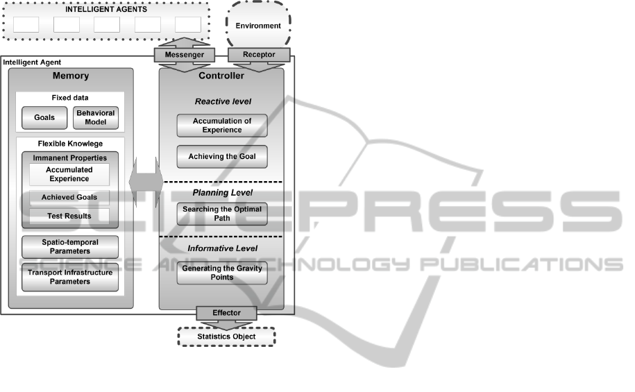
Refer to figure 1 to see the architecture of the in-
telligent agent from the set A
I
. The designed archi-
tecture allows agents to interact with each other and
with the environment, which changes are not prede-
fined.
Figure 1: Intelligent agent architecture.
The architecture of an intelligent agent is repre-
sented by the following structural units: a controller,
a memory, the means of communication with the
environment (receptor, messenger and effector), and
the means of interaction between these blocks.
The receptor receives information from the envi-
ronment, and determines further action on its pro-
cessing and stores the required data in the memory.
The effector collects information about the gravi-
ty points P
A
(Mikheeva, 2014) during the modeling
object process. The collected information is used by
the statistics gathering object. At the end of each
reporting period ∆t, which corresponds to a calendar
day, the agent a
I
i
generates a report, which repre-
sents a dataset containing the following data:
 p
opt
i
- the selected optimal path;
 t
opt
- the time spent to complete the optimal
path p
opt
i
;
 p
A
i
- the list of gravity points with the values
of their load u
A
i
.
The messenger is designed for communication
between intelligent agents and provides composing,
sending, and receiving messages.
The memory unit is used to store the collected
data. There are two memory blocks: area of the fixed
data (obtained at initialization), and the area of the
flexible knowledge (data changed during processing
by the agent).
The controller provides data processing, gener-
ates reactions according to the data received from
receptors and messengers, solves problems, and
generates data for the effector. The agent’s control-
ler is divided into three planning levels: reactive and
informative.
At the planning level agents a
I
i
are initialized ac-
cording to one of the driver models M
beh
(Gonzalez,
2008). Determination of the scope occurs according
to the selected model m
beh
(a
I
i
)∈M
beh
, which depends
on the SRN model, and the results of calculation of
the optimal route by the SRN graph G’=(V’,E’)
according to the assigned chain of correspondences.
The problem of navigating through the SRN
graph G’ is solved by considering the individual
driver behavior model m
beh
(a
I
i
) at the reactive level.
The task of processing the signals from the receptor
and the messenger is also resolved at this level. The
reactive subsystem is based on neural network tech-
nology, which matches typical situations in the envi-
ronment with the reaction of agents’ behavior. This
approach allows making effective decisions while
the intelligent agents move along the street and road
network graph.
The informative level is a neural network train-
ing process. The neural network accumulates
knowledge about dislocation and load values in the
gravity points P
A
.
The proposed architecture of an intelligent agent
provides necessary qualities of its behavior, such as
complexity, autonomy and intelligence. It is
achieved by using a neural network in an intelligent
agent adapted to working in a transport infrastruc-
ture modeling environment.
3 MICROSCOPIC TRANSPORT
SIMULATOR
3.1 Simulator Mathematical Model
Data generated by the simulation of a traffic flow
includes amount, dislocation, and load values of
gravity points of a city. The modeling object A
M
is
used for traffic simulation, which generates the fol-
lowing objects: the coordination object, the statistics
object, and the set of intelligent agents
A
I
={a
I
1
,…,a
I
N
}. The listed objects are represented in
the common environment E and interact with each
other.
MultilevelModellingofUrbanTransportInfrastructure
79

The coordination object is used for the manage-
ment of intelligent agents A
I
={a
I
1
,…,a
I
N
}. The coor-
dination object determines the creation time and the
time of achieving the set goals for each agent a
I
i
,.
The coordination object performs the accounting of
time in the following format: “season”, “day of
month”, “weekday”, “hour” (Kravets, 2013).
The statistics object is used to predict the tension
on the parts of the SRN.
The mathematical model of the modeling object
A
M
is as follows:
{}
APE
out
IM
FMSAEA ,,,,=
(1)
where E - is a finite set of objects in the envi-
ronment, including the SRN model objects and
transport infrastructure;
A
I
={a
I
1
,…,a
I
N
} is the finite set of intelligent
agents, that are represented by an extended mathe-
matical model;
S
E
out
– the set of states of the environment E;
M
P
– a set of traffic laws;
F
A
– a set of functions describing the changes in
the state of transport infrastructure (Saprykina,
2013).
3.2 Simulator Implementation
Analysis of the street and road network configura-
tion is performed by the use of simulation tools
based on freeware component library MATSim
(Multi-Agent Transport Simulation) (Rieser, 2014).
Modeling objects designed in the previous sections
are created in the MATSim environment by extend-
ing the built-in classes. For example, a MATSim
agent class is extended to the developed intelligent
agent. Intelligent agents act as mini-systems in-
volved in continuous interaction with each other,
and are capable of independent actions. Agents are
coordinated and their actions are structured accord-
ing to the current objectives.
The system contains the following functional
blocks:
 micro-modeling simulation of the transport
flow;
 collection and processing of the simulation
process data;
 dynamic visualization of the simulated pro-
cess.
A city map is converted from OpenStreetMap
format to the MATSim internal format. The model
of a map is a sequence of road sectors, each contain-
ing the following immanent properties: capacity;
maximum allowed speed of movement; number of
lanes in the SRN area; direction of movement; road
surface quality.
The MATSim core calculates routes of agents’
movement at a given time, with all the street and
road network attributes. While moving about the
map agents update their state and collect traffic
congestion and tension data storing it in a database.
During the simulation in the output folder files are
created with the results that contain the full path and
travel time of each agent.
The simulation result can be reviewed by upload-
ing files obtained in the previous step into a dynamic
visualization unit (Fig. 2). The subsystem allows
seeing the distribution of agents over time, tracking
problematic time intervals and areas of the city and
figuring out gravity points.
Figure 2: Visualising the process of microsimulation.
Agents are having speed, which close to the free
speed route, are highlighted in green while modeling
the transport process. The red color indicates traffic
congestions. Figure 2 shows traffic congestions on
major highways of the Samara city at the evening
rush hour. The simulation results match the actual
situation on the street and road network of the city,
as confirmed by field studies and the data of traffic
information web services.
4 TRANSITION TO
MESOSCOPIC LEVEL
Tension, density, and intensity in certain SRN areas
are represented at the mesoscopic level of the city
transport model (Kerner, 2009). Let us review the
construction of the tension function of the gravity
points using the data obtained at the microscopic
level. The statistics gathering object uses a neural
network. Training of the neural network is per-
formed during the intelligent agents’ a
I
i
moving on
the SRN graph G’ according to the set of rules (in-
VEHITS2015-InternationalConferenceonVehicleTechnologyandIntelligentTransportSystems
80

telligent function). Each intelligent agent a
I
i
dynami-
cally trains the neural network throughout its life
cycle. A trained neural network is able to predict
tension values at any given gravity point.
The neural network used in the statistics object is
a three-layered Ward neural network, which is capa-
ble of conducting a qualitative analysis by allocating
the initial data in various aspects. This is achieved
by a special type of neural network architecture, a
hidden layer which is divided into several blocks. In
this case each block has its own transfer function
that facilitates the parallel processing of signals
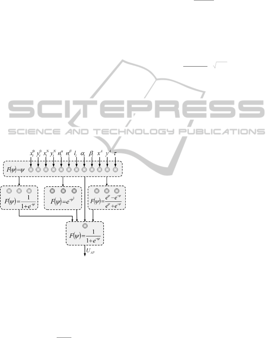
received from the input layer. Architecture of the
Ward neural network is shown in Figure 3. The
input layer of the neural network consists of the
following parameters: (x
A
, y
A
) - coordinates of a
gravity point, (x
0
, y
0
), (x
N
, y
N
) - coordinates of the
beginning and the end of the arc of the graph corre-
sponding to the SRN section, l
i
- length of the SRN
section, n
α
i
- number of lanes on an SRN section in
the forward direction, n
β
i
- number of lanes on SRN
section in the opposite direction, α - rotation angle of
the forward direction, β - rotation angle of the oppo-
site direction, τ – temporal parameters.
Figure 3: Architecture of the Ward neural network.
A linear activation function F(ψ)=ψ is used for
the input layer of the Ward neural network. The
number of neurons in the input layer is dictated by
the number of variables. The hidden layer is repre-
sented by the three blocks. Activation functions for
the hidden layer units are chosen experimentally,
which are:
 sigmoid:
()
ψ
ψ
−
+
=
e
F
1
1
(2)
 hyperbolic tangent:
()
ψψ
ψψ
ψ
−
−
+
−
=
ee
ee
F
(3)
 radial basis:
()
2
ψ
ψ
−
= eF
(4)
A sigmoid activation function is used at the out-
put layer. The number of neurons in the hidden layer
is calculated as follows:






+
+
=
exphidden
2
N
NN
N
outin
(5)
where:
N
in
-is the number of neurons in the input layer
(N
in
=11);
N
out
- is the number of neurons in the output layer
(N
out
=1);
N
exp
- is the number of the performed experi-
ments (Rutkovskaya, 2004).
Ward neural network training is performed by
backpropagation. Selection of weighs occurs every
time when applying tension information u
A
i
∈U at the
gravity point p
A
i
obtained from the agent a
I
i
∈A
I.
while transferring the data to the neural network.
Thus, the statistics object shows the dependence
of the temporal and spatial characteristics of the
investigated area on the tension u
A
i
∈U of gravity
points p
A
i
∈P
A
. The resulting neural network is capa-
ble of storing the data obtained at the microscopic
level and solving transportation problems on
mesoscopic and macroscopic levels.
5 CONCLUSIONS AND FUTURE
WORK
This article describes the modified microscopic
traffic simulator with agents figuring out knowledge
about SRN bottlenecks to transfer to a higher model-
ing level. This information is used at the mesoscopic
level to train the neural network, which allows keep-
ing hidden patterns in the form of synaptic connec-
tions. The discovered dependencies allow analyzing
the modified transport infrastructure without running
additional simulation cycles.
The work on constructing models of transition
from mesoscopic to macroscopic parameters allow-
ing finding the optimal structure of street and road
network is underway.
MultilevelModellingofUrbanTransportInfrastructure
81

ACKNOWLEDGEMENTS
This work is supported by a grant from Samara State
Aerospace University.
Special thanks to Professor T.I. Mikheeva for as-
sistance in methodology of transport infrastructure
description.
REFERENCES
Shahin, M.M., 2012. Traffic congestion propagation at
road bottlenecks in developing countries. In Traffic
Engineering and Control, 53(4). Pp. 137-143.
Gregoriades, A., Mouskos, K. and Michail, H., 2012. An
Intelligent Transportation System for Accident Risk
Index Quantification. In Proceedings of the 14th In-
ternational Conference on Enterprise Information Sys-
tems. SciTePress. Pp. 318-321.
Cavar, I., Petrovic, M., Vujic, M., 2013. Microscopic
simulation of a multimodal urban traffic network. In
Proceedings of the 11th International Industrial Simu-
lation Conference, ISC 2013. Ghent, Belgium. Pp.
240-242.
Savrasovs, M., 2011. Urban transport corridor mesoscopic
simulation. In Proceedings of the 25th European Con-
ference on Modelling and Simulation ECMS 2011.
Dudweiler, Germany. Pp. 587-593.
Burghout, W., 2004. Hybrid microscopic-mesoscopic
traffic simulation. Royal Institute of Technology
Stockholm, Sweden.
Kolosz, B.W., Grant-Muller, S.M.; Djemame, K., 2014. A
Macroscopic Forecasting Framework for Estimating
Socioeconomic and Environmental Performance of In-
telligent Transport Highways. In IEEE Transactions
on Intelligent Transportation Systems, 15(2). IEEE,
England. Pp. 723-736.
Gaud, N., Galland, S., Koukam, A., 2008. Towards a
Multilevel Simulation Approach based on Holonic
Multiagent Systems. In Proceedings of the 10th Inter-
national Conference on Computer Modelling and
Simulation. IEEE, England. Pp. 180–185.
Kumar, P., Merzouki, R., Conrard, B., Coelen, V., Ould
Bouamama, B., 2014. Multilevel modeling of the traf-
fic dynamic. In IEEE Transactions on Intelligent
Transportation Systems, 15(3). IEEE, England. Pp.
1066-1082.
Russell, S., Norvig, P., 2010. Artificial Intelligence: A
Modern Approach. Prentice Hall. New Jersey, 3rd Edi-
tion.
Mikheeva, T.I., 2014. Intelligent transport system: meth-
od, algorithms, realization. LAP LAMBERT Academ-
ic Publishing. Deutschland, Germany.
Gonzalez, M., Hidalgo, C., Barabasi, A., 2008. Under-
standing individual human mobility patterns. In Na-
ture, Vol. 453. Pp. 779-782.
Kravets, A.D., Fomenkov, S.A., 2013. Development of
Multi-Agent Systems Agent Generationmodel. In In-
novative Information Technologies. Pp. 270-273. (In
Russ.).
Saprykina, O.V., Saprykin, O.N., Sidorov, A.V., 2013.
The transport network evolution model. In Proceed-
ings of the 15th International Workshop on Computer
Science and Information Technologies (CSIT'2013).
Information Scientific Issue, Ufa. Pp. 86-88.
Rieser, M., et al., 2014. MATSim User Guide.
http://www.matsim.org/
Kerner, B., 2009. Introduction to modern traffic flow
theory and control. Springer. Berlin.
Rutkovskaya, D., Pilinskiy, M., Rutkovskiy, L., 2004.
Neural Networks, Genetic Algorithms and Fuzzy Sys-
tems. Goryachaya liniya Telekom. Moscow. (In
Russ.).
VEHITS2015-InternationalConferenceonVehicleTechnologyandIntelligentTransportSystems
82