
Fault Detection Architecture for Proprioceptive Sensors based on a
Multi Model Approach and Fuzzy Logic Decisions
Nicolas Pous
1
, Dominique Gruyer
2
and Denis Gingras
1
1
LIV (Laboratory of Intelligent Vehicles), in the Electrical and
Computer Engineering Department of Sherbrooke University, Sherbrooke, Qc J1K 2R1, Canada
2
IFSTTAR- IM - LIVIC, 14 route de la minière, bat. 824, 78000 Versailles-Satory, France
Keywords: Failure Detection, Intelligent Vehicle, Localization, Data Fusion.
Abstract: In this paper a new fault detection architecture will be presented. Inspired by multi-model data fusion
algorithms and fuzzy logic decisions, it consists in the comparison between the estimation of a dynamic mode
using each sensor independently. This method is used to deal with important non-linearity and strong
interaction with the environment usually encountered in the domain of the intelligent vehicles localization.
The concept of analytic redundancy is also used to ignore model uncertainties.
1 INTRODUCTION
More and more, our society is evolving to be partially
automatized. In this context, the automotive industry
is contributing by focusing on autonomous vehicles.
As a step between this technology and the previous
one, vehicular companies are developing a large
series of tools helping drivers and improving both
safety and comfort. These tools, when used to
improve driving safety, are generally named ADAS
(Advance Driver Assistance System) (Andreas
Riener, 2009). ADAS are generally composed of a
large amount of tools permitting, for example, to
reduce stopping distance, or improve the car position
determination. In that case precisely, a large set of
exteroceptive and proprioceptive sensors are used to
obtain a better knowledge of the vehicle environment
and attitude, in order to reduce the localization
uncertainties via data fusion algorithms. Some of
them are using only proprioceptive sensors (Cai Bai-
gen et al., 2009), others are using both (Kim, S.-B et
al., 2011 and Adrien Bak et al., 2012).
Communication and map matching can also be used
to reinforce the precision of the measurement (Rohani
et al., 2013 and Rohani et al., 2014).
In both cases, a faulty data source can lead to a
catastrophic error in the position determination.
That’s why, in order to properly improve safety, we
need to detect faults and identify the associated
sources before using faulty data in the fusion
algorithm. One of the most used detection method is
based on the comparison between the normal
behavior model and the recording of the real behavior
from the sensors. This method supposed that the
system behavior is perfectly known and can be
modeled (Patton, R. J. et al., 1989).
But, the important non-linearity of our system (The
vehicle) behavior and the strong impact of
environmental perturbation will improve the
complexity of our task. Others methods based on
analytical redundancy are also used to avoid the
model issues, as described in (Sun and Cannon,
1998), where a Kalman filter is used to obtain
estimations of a same metric in order to compare the
values obtained from different sensors.
In this paper an alternative approach based on the
determination of the dynamic comportment of the
vehicle using analytical redundancy is developed in
order to treat with the non-linearity of the system. The
nominal comportment was divided in 4 sub-systems
defined by the direction changes and longitudinal
accelerations as describe in table 1.
Table 1: Dynamic modes definition.
Straight line H1 H3
Speed change H2 H4
Based on the sensors information, we will use fuzzy
logic and calculate the weight corresponding to the
membership degree of each dynamic mode in every
time, and use these values from each sensor to
determine the presence of a faulty data source.
25
Pous N., Gruyer D. and Gingras D..
Fault Detection Architecture for Proprioceptive Sensors based on a Multi Model Approach and Fuzzy Logic Decisions.
DOI: 10.5220/0005459700250032
In Proceedings of the 1st International Conference on Vehicle Technology and Intelligent Transport Systems (VEHITS-2015), pages 25-32
ISBN: 978-989-758-109-0
Copyright
c
2015 SCITEPRESS (Science and Technology Publications, Lda.)

In part 2 a traditional approach for the fault detection
will be studied and our context will be presented.
Then, in part 3, the proposed method based on the
dynamic mode determination will be presented.
Section four will then present some simulation results
and a performance analysis before treating in the fifth
section of the ongoing developments and conclude in
section six.
2 CONTEXT AND TRADITIONAL
APPROACH
2.1 Context
As we focused on the ego-localization of an
intelligent vehicle, we decided to focus on
proprioceptive sensors related to the vehicle
comportment determination.
2.1.1 Odometer
The odometer is based on an electric sensor detecting
marks equally disposed on a wheel. As the odometer
is a counting device, the output will be a discrete
value representing both the integrated travelled
distance and the speed during a sampling time.
2.1.2 INS
The INS is usually composed with 3 accelerometers
and 3 gyroscopes which respectively provide
information about linear accelerations and angular
speed on the 3 axes.
2.1.3 Compass
The compass, usually integrated on the INS chip, will
inform us about the absolute orientation of our
mobile.
2.1.4 GNSS
This device provide the absolute position of the
vehicle on the earth.
2.2 Traditional Approach
Traditionally, a system and the associated FDI (Fault
Detector and Identification) are represented as
followed. In this representation, we can distinguish
three parts which can present faults. The actuators,
the system itself and the sensors which give
information about the system comportment.
Figure 1: Classical structure of an FDI model based.
(Qi et al., 2013) present a description of the different
eligible faults on the actuators, the system and the
sensors. According to these description, we can
elaborate tests to detect every kind of fault, for every
part of the complete data flow (Actuators, System, in
our case, the vehicle and Sensors) as describe in
figure 1. Here, as we focus in this publication on the
sensors faults, actuators and system failures and
uncertainties will not described.
Four types of faults are depicted by Qi et al. for the
sensors.
- Total failure
- Constant bias failure
- Constant gain failure
- Outlier failure
Knowing these failures nature, we can elaborate tests
to detect the presence of each kind of failure. Usually,
model-based fault detector assume that at least one
part of the global system (representing the system
with its actuators and sensors) is working efficiently.
In this paper we will discuss about new techniques to
detect and identify faults without any assumptions on
any part of the global system. In that purpose, we
developed a detection method based on the
information redundancy and determination of the
system comportment.
3 DYNAMIC MODE
DETERMINATION
Inspired by the IMM fusion algorithm presented in
(Gruyer et al., 2010), we developed a multi-model
approach to detect faulty behavior on sensors used in
the determination of a mobile position. The multi-
model implementation consists in separating the
operating space into linear sub-spaces where we can
identify some simple maneuvers. This sub-space, also
called dynamic mode, has then to be determined only
VEHITS2015-InternationalConferenceonVehicleTechnologyandIntelligentTransportSystems
26

using the sensors data. The determinations from
different sensors will so diverges if one of them
present a faulty comportment.
The global structure of our fault detection and
identification architecture is depicted in figure 2.
Figure 2: Proposed FDI structure.
The dynamic modes are defined by the longitudinal
acceleration and the angular velocity of the mobile
(representing the two possible maneuvers for the
user), and we so can separate the operating space into
four principle dynamic modes as seen in Table 1.
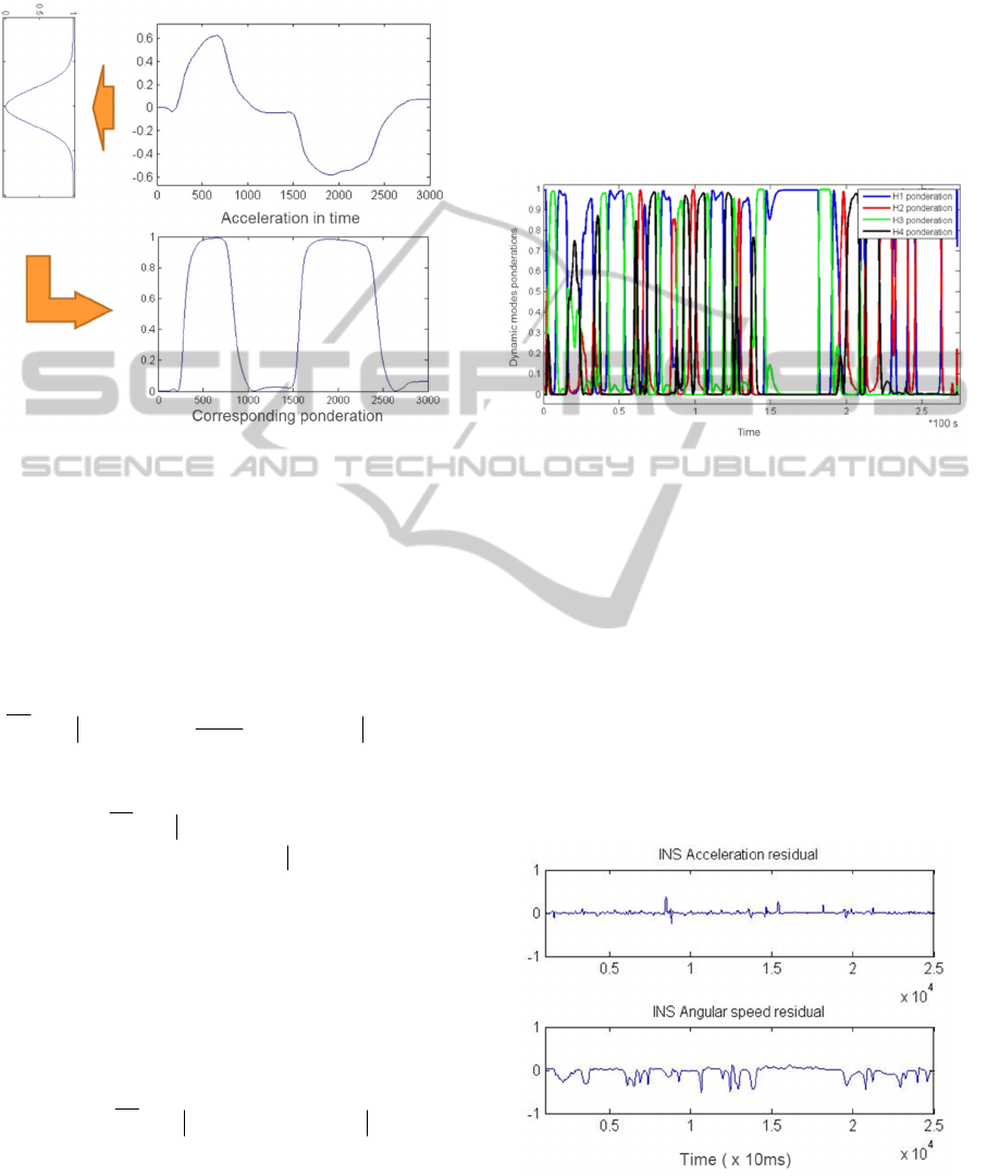
Figure 3: Acceleration and angular speed distribution for
the four dynamic modes.
According to the dynamic mode description, the two
needed metrics are the acceleration and the angular
speed of the vehicle.
3.1 Metrics Determination
So we need to determine these two characteristics
using each sensor independently. Concerning the
INS, these two values will be directly given by the
sensor. Concerning the odometer, it is necessary to
recalculate the value according to the nature of the
information given by the sensor. As we have the
speed of each wheel from the odometer, we can
approximate the speed of the vehicle (VE_S) by
computing the mean value of the right and left wheels
speed.
(1)
Where RW_S and LW_S are the right and left
wheel speeds respectively. It is now possible to
determine the acceleration by deriving the speed
value.
(2)
Having the acceleration, we need now to
determine the angular speed of the vehicle. In order
to determine if we are in a straight line or in a curve,
we analyze the differential speed between the 2
wheels given by (3).
(3)
Concerning the compass, it can only inform us
about the angular speed, by derivation of the
orientation θ(t).
(4)
3.2 Weight and Residual
Determination
Knowing acceleration and angular speed values, it is
now possible to determine the dynamic mode. Let’s
call Acc the presence of an acceleration, and Vθ the
presence of a rotation, so the 4 dynamic modes will
be defined as follow.
(5)
Instead of a classic determination using a simple
threshold, a fuzzy logic decisions permit to determine
a weight corresponding to the presence of an
acceleration/rotation, as represented in figure 4 for an
acceleration. The event probability is currently
determine using a Gaussian threshold as depicted in
equation 6 for the presence of an acceleration, where
the σ coefficient value permit adjust the sensitivity if
the detector.
(6)
(7)
_
() _ ()
_()
2
R
WSt LWSt
Ve S t
(_()) _() _(1)
()
Odo
DVESt VESt VESt
Acc t
Dt T
_() _() _()
Odo
DifS t RWSt LWSt
()
_()
Compass
t
An Sp t
t
1
2
3
4
HAccV
HAccV
HAccV
HAccV
2
0.5*( / )
0.5
1
1*
(0.4 * (2 * )
INS
Ac
Acc
c
expP
pi
1
2
3
4
(1 ) * (1 )
*(1 )
(1 ) *
*
HAccV
HAcc V
HAccV
HAccV
P
PP
PP P
PPP
PPP
FaultDetectionArchitectureforProprioceptiveSensorsbasedonaMultiModelApproachandFuzzyLogicDecisions
27
Then, the dynamic mode membership degree can
be determined as followed, where Px is the weight
corresponding to the event x.
Figure 4: Acc Weight’s determination according to the
acceleration value.
Using these weights from each sensor, it is
possible to determine an instantaneous mean value of
the corresponding metric weight by using equation
(8) taking into account every sensors independently.
Instead of calculating dynamic mode weights, we
dissociate the 2 metrics weights (Po(Acc) and
Po(Vθ)) which will be more useful.
(8)
Where is the mean value
taking all the sensors, is
the acceleration weight for the sensor
i, and C
i
corresponding to the decision of the fault
detection device.
Using both the mean weight value and individual
ones, we can calculate a residual value for each sensor
equal to the difference between the two of them (9).
A residual variable will then be calculated for each
sensor and each metric used (acceleration and angular
speed).
(9)
The calculated residual has to be stationary to
make the detection easier. In our case, for a normal
behavior, the residual variable will have a zero mean
value. In order to illustrate it, we simulate the drive of
a vehicle with the appearance of the 4 dynamic
modes, with only the use of four odometers (one on
each wheel, simulated by the recording of the wheel
speed), and an inertial system with accelerometers
and gyroscopes on the three axes. The figure 5
represents the mean weight calculated with
information of all the sensors, and figure 6 is the
residual variable for both acceleration and angular
speed for the inertial sensor.
Figure 5: Dynamic modes weights evolution in time.
These results were obtained by calculating the
differential weight between the mean weight values
and the INS ones. As the sensors information was
noisy, we decided in a first time to apply a
Butterworth low pass filter to eliminate the high
frequencies component of signals.
The residual value is still not perfect, and some
adjustment are still needed, but it remains possible to
use these results for the detection algorithm. Actually,
what is primordial is to observe modification of the
residual values, so, it’s possible to imagine calibration
procedure to determinate a standard residual profile
before beginning the analysis.
Figure 6: Acceleration and angular speed residual for the
INS sensor.
12
1
1
1
( , ... ) ( )
N
Nj
N
j
j
i
i
P
o Acc S S S C Po Acc S
C
12
( , ) ( , ... ) ( )
iNi
RAccS PoAccS S S PoAccS
12
( , ... )
N
Po Acc S S S
()
i
P
oAccS
VEHITS2015-InternationalConferenceonVehicleTechnologyandIntelligentTransportSystems
28
3.3 Fault Detection
In this section, faulty data will be introduce in sensors
information, according with what was described in
section 2-c, regarding the sensors faults. We so
simulated each kind of fault and analyzed the residual
values in order to establish some detection rules. Just
as we did previously in this section, we will focus on
two kind of sensors, odometers (one on each wheel)
and inertial system.
As depicted in the previous section, the residual
will be calculated by computing the difference
between the mean weight value and the weight from
the sensor under watching. But as a failure will induce
some perturbation on the mean value calculation, it’s
important to determinate how this perturbation will
impact the failure detection. Considering a
perturbation ΔPo on one sensor noted S
F
, the mean
weight value, before the decision can be represented
by equation 10.
(10)
The residual of a non-faulty sensor will so be
impacted by a failure, and this impact will depend on
the number N of sensors used in the detection
algorithm. Residuals for both faulty and non-faulty
sensors can so be calculated by (11) and (12), and the
related perturbations can so be depicted by (13) and
(14), where N is the number of sensors used in the
mean value calculation.
(11)
(12)
(13)
(14)
The more sensors we use, the more important the
difference between a non-faulty and a faulty residual
will be. This also mean that it is important to
distinguish by comparison, a perturbation on the
residual due to another sensor fault.
4 SIMULATIONS AND
PERFORMANCE ANALYSIS
All the simulation were realized with the help of the
ProSivic simulator, which permit to simulate the
dynamic behavior of a vehicle, and the real reaction
registered by the sensors. This simulator allow us to
determine the trajectory and the speed of a vehicle
and will return us all the others component of the
mobile state, like position, acceleration, angular
speed…
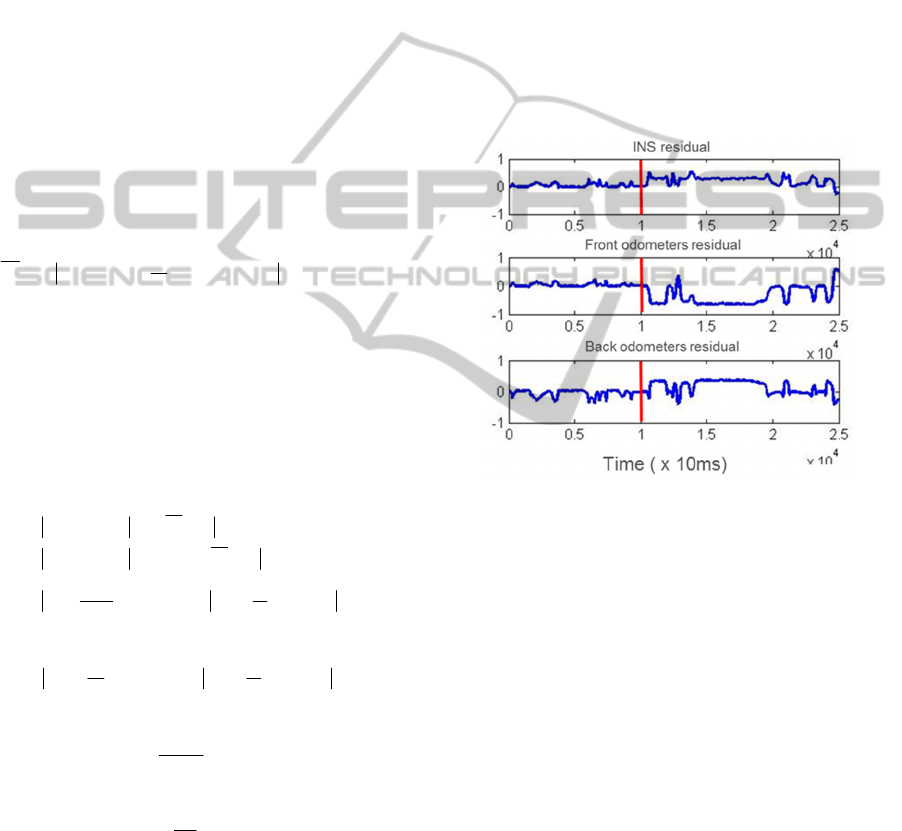
In order to illustrate the response to a faulty
comportment, a gain on the speed measurement of the
left front wheel has been injected to simulate a failure,
100 seconds after the beginning of the simulation.
Figure 7: Comportment of residuals with the introduction
of a faulty comportment on one of the sensors.
Figure 7 presents the residuals for respectively the
INS, the front and the back odometers for the angular
speed determination. As predicted, the amplitude of
the residual value is increasing after the injection of a
failure, and the most important raise coming from the
affected sensor. It also appears that the residual of the
faulty sensor is the opposite of the others sensors as
prove equations (11) and (12). As the appearance of a
failure will create an event different for each type
(Detecting a rotation in a straight line mode, an
acceleration in a constant speed mode) but will
remain undetectable during some dynamic mode. It’s
so important to go through every dynamic mode to be
sure to detect failures. For example, a failure on an
odometer as presented previously will introduce a
rotation even if the real dynamic mode is descripting
a straight line. But if the vehicle remains in a rotation,
the detection cannot be done. A better way is to
analyze the mean values of all the residual on a long
12
1
1
(,...) ()
N
Nj
j
j
Po Acc S S S C Po Acc S Po
N
12
12
1
( ) ( ) ( , ... )
()( ) (,...)
11
() ( ) ()
FF N
FNF N
N
FNFi
i
R Acc S Po Acc S Po Acc S S S
R Acc S Po Acc S Po Po Acc S S S
N
R
Acc S Po Po Acc S Po Acc S
NN
1
11
() () ()
N
NF NF i
i
R
Acc S Po Po Acc S Po Acc S
NN
1
F
N
RPo
N
1
NF
RPo
N
FaultDetectionArchitectureforProprioceptiveSensorsbasedonaMultiModelApproachandFuzzyLogicDecisions
29
time period with the occurrence of all the dynamic
mode in order to realize the detection.
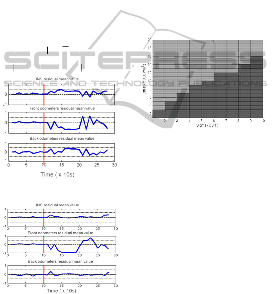
We can observe in figure 8 that the mean value of
each residual is varying according to equation (13)
and (14), but it’s necessary now to determine decision
laws to minimize the false alarms and missed
detections rate. The optimization will be part of the
future work. For now, we assume that the detection is
decided by a threshold determined analytically at 0.4.
In that case, after the detection the faulty data source
will not be taken into account in the mean value
computation, just as described in equation (9) where
the corresponding decision coefficient C will be equal
to 0. The residual of a non-faulty and a faulty sensor
will so be as described respectively in equation (15)
and (16).
12
( ) ( ) ( , ... )
NF NF N
R Acc S Po Acc S Po Acc S S S
(15)
12
( ) ( ) ( , ... )
FNF N
R Acc S Po Acc S Po Po Acc S S S
(16)
Figure 8: Residual mean value calculated every 10 seconds
for each sensor.
Figure 9: Residual mean value taking into account the
decision procedure.
The perturbation for a non-faulty sensor will so be
zero centered while the perturbation for a faulty one
will correspond to the perturbation on the weight
ΔPo.
As predicted, incorporating the decision process
will keep the non-faulty residuals around zero and
increase the faulty residual value.
A second set of simulations has been run in order
to illustrate the detection of a failure corresponding to
an offset appearing on the acceleration given by the
INS. In these simulations we varied both the offset
values and the threshold sensitivity σ to study their
impact on the fault detection. Figure 10 present the
results of the fault detection according to σ and the
offset value.
Figure 10: Fault detection according to sigma and offset
value.
The red zone correspond to a good fault detection,
and the blue correspond to a missed detection. It’s so
possible to see that reducing the σ value permit the
detection of smaller faults. But, reducing this value
will also mean that the fault detector will be more
sensitive to noise. A simulation with different noise
levels has also been realized in order to study this
sensitivity. A white noise was so injected on the INS
measurement only, with an RMS value varying from
0.01 to 0.2 m/s2. A new set of simulation was run,
keeping an offset of 0.5 m/s2 (100 seconds after the
beginning of the simulation) and varying the sigma
value from 0.1 to 1 (just like the previous simulation
set).
During the first part of the simulation, when the
fault has still not appeared, the presence of noise can
create some false alarm when the sigma value is too
low.
After the appearance of the offset, the algorithm
is working efficiently. As the injected offset is set at
0.5 m/s2, the minimum sigma value needed for the
detection will be around 0.5 (as shown by the
previous study, figure 10). It seems logical to expect
VEHITS2015-InternationalConferenceonVehicleTechnologyandIntelligentTransportSystems
30
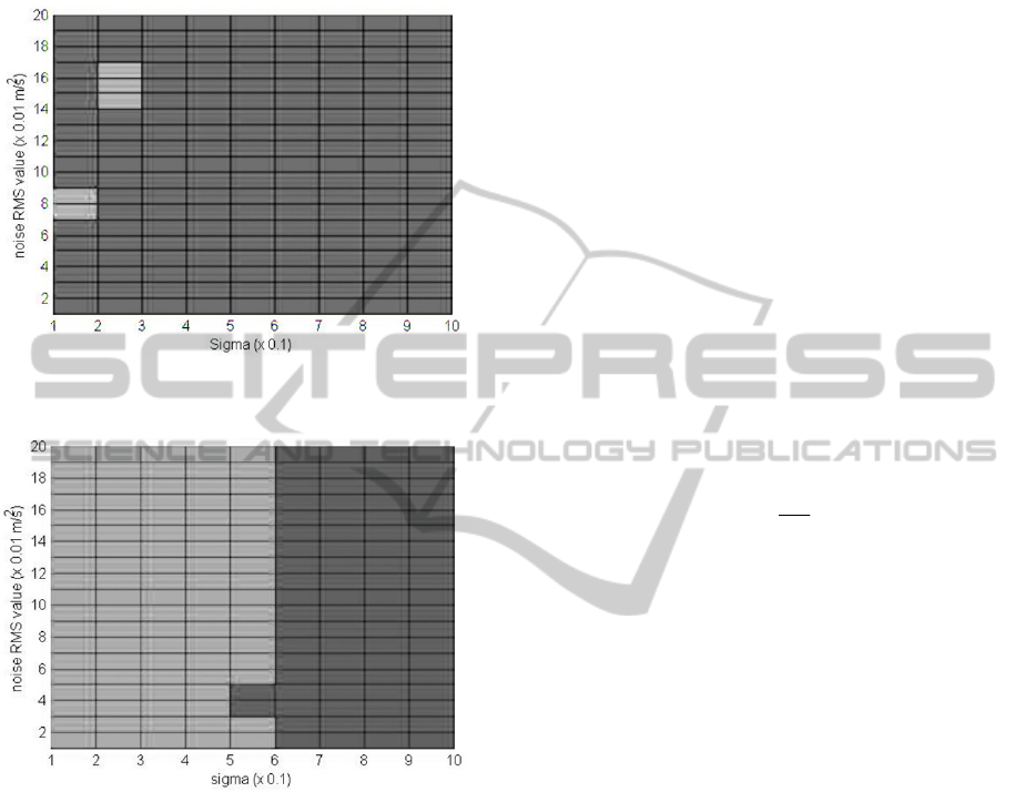
a detection for the sigma values below 0.5 while there
will be no detection for the upper values. This is
verified in this simulation (figure 12) where the
detection is realized for the lower sigma values.
Figure 11: false alarm due to noise when sigma value is too
low.
Figure 12: Offset detection with different sigma values
varying noise level.
These results verify what has been said earlier, the
detection is well done for a sigma value lower than
0.5, for every noise level injected.
For now, the residuals generated permit the
distinction of most of the default presented in the
section 2, but not all of them. It is still necessary to
work on the residual analysis and on others residuals
to be able to detect and identify all kind of faults.
5 FUTURE WORK
As it was said in the previous section, the analysis of
residuals will lead to the failure detection, and the
distinction of which sensor is faulty. But, in our
problematic, it’s also important to distinguish faults
generated by sensors to other ones due to
environment interferences or a system perturbation
(flat wheel…). So, we need to develop strategies to
establish the distinction between each kind of fault.
To bring out this strategy, let’s discuss about a
concrete case, and compare the results obtained for
three different faults.
We imagined a scenario where a fault on one of
the odometers appears. This fault is traduced by a
gain on the distance measured as described in (17).
(17)
Dist
Me
is the measures distance, Dist
Real
is the real
distance and x is the number of marks originally
presented on the encoded wheel. This kind of fault is
generally caused by a missing mark on the coded
wheel. It’s corresponding to a contact gain failure, as
depicted in the second section concerning sensors
failures. But, a flat tire could also have an equivalent
impact, as the wheel diameter will be reduced, with a
same angular speed, the travelled distance will be
smaller.
(18)
Where
D
iF
and D
iN
are respectively the flat tire
and the normal wheel diameter. Mathematically these
two errors lead to the same result, but it remains
important to be able to distinguish the two of them. In
the future work we will focus on this distinction by
using a three dimensional model of our system.
6 CONCLUSIONS
This first paper is a presentation of the architecture
and preliminary results on the fault detection method
proposed.
In this paper a new fault detection architecture was
presented, based on a multi-model approach. In a first
time, our context was presented before introducing
the developed method using both a multi –model
approach and a fuzzy logic decision to generate
residual variables allowing to distinguish faulty data.
As explained in the section 3, the residual will permit
to detect perturbation by computing the difference
between weights of each sensor independently and a
mean value computed with all the sensors. It also has
been demonstrated that adding the decision result to
the mean value computation will increase the
difference between a faulty and a non-faulty residual,
which permit a better discrimination between the two
of them.
Re
(1 1 / )
Me al
Dist Dist x
Re
iF
Me al
iN
D
Dist Dist
D
FaultDetectionArchitectureforProprioceptiveSensorsbasedonaMultiModelApproachandFuzzyLogicDecisions
31

In the simulation results presented in the section
four, two study cases have been presented. The first
one corresponding to a gain on the odometer speed
allowed us to illustrate the calculation proposed on
the previous section, and so to verify the efficiency of
the proposed FDI. Finally, a study on the sensitivity
and robustness has been effected on the second case,
presenting an offset on the INS acceleration. This
study also permit to determine the importance of the
detector parameters configuration according to the
noise and the needed sensitivity.
ACKNOWLEDGEMENTS
This work is part of CooPerCom, a 3-year
international research project (Canada-France). The
authors would like to thank the National Science and
Engineering Research Council (NSERC) of Canada
and the Agence nationale de la recherche (ANR) in
France for supporting the project STP 397739-10.
REFERENCES
Andreas Riener; 2009; Sensor-Actuator Supported Implicit
Interaction in Driver Assistance Systems; Chapter 9;
vieweg-teubner.
Cai Bai-gen; Wang Jian ; Yin Qin ; Liu Jiang, 2009, A
GNSS Based Slide and Slip Detection Method for Train
Positioning, Asia-Pacific Conference on Information
Processing, APCIP 2009.
Kim, S.-B.; Bazin, J.-C.; Lee, H.-K.; Choi, K.-H.; Park, S.-
Y.; 2011; Ground vehicle navigation in harsh urban
conditions by integrating inertial navigation system,
global positioning system, odometer and vision data;
Radar, Sonar & Navigation; Vol.5; pp 814 – 823.
Adrien Bak; Dominique Gruyer; Samia Bouchafa; Didier
Aubert; 2012; Multi-Sensor Localization – Visual
Odometry as a Low Cost Proprioceptive Sensor; ITSC.
Rohani, M.; Gingras, D.; Vigneron, V.; Gruyer, D., 2013;
A New Decentralized Bayesian Approach for
Cooperative Vehicle Localization based on fusion of
GPS and Inter-vehicle Distance Measurements;
ICCVE.
M. Rohani; D. Gingras; D. Gruyer, 2014; Vehicular
Cooperative Map Matching; International Conference
on Connected Vehicles and Expo (ICCVE).
Patton, R.J; Frank, P.; Clark, R.; 1989; Fault Diagnosis in
Dynamic Systems, Theory and Application; prentice
hall.
Xin Qi; Didier Theilliol; Juntong Qi; Youmin Zhang;
Jianda Han, 2013; A Literature Review on Fault
Diagnosis Methods for Manned and Unmanned
Helicopters; International Conference on Unmanned
Aircraft Systems; May 28-31.
Gruyer, D.; Pechberti, S.; Gingras, D.; Dupin, F.; 2010,
Robust positioning in safety applications for the CVIS
project; IEEE Intelligent Vehicles Symposium; pp 262 -
268.
Mr. Huangqi Sun; Dr. M. Elizabeth Cannon, 1998;
Relibaility analysis of an ITS navigation system;
Department of Geomatics Engineering; The University
of Calgary; Calgary, Alberta, Canada.
VEHITS2015-InternationalConferenceonVehicleTechnologyandIntelligentTransportSystems
32
