
Blood Flow Prediction and Visualization within the Aneurysm of the
Middle Cerebral Artery after Surgical Treatment
Artem M. Yatchenko
1
, Andrey V. Gavrilov
1
, Elena V. Boldyreva
2
, Ivan V. Arkhipov
3
,
Elena V. Grigorieva
4
, Ivan M. Godkov
4
and Vladimir V. Krylov
4
1
Lomonosov Moscow State University, Moscow, Russia
2
Institute of Machines Science named after A. A. Blagonravov of the Russian Academy of Sciences, Moscow, Russia
3
Petrovsky National Research Center of Surgery of Russian Academy of Medical Sciences, Moscow, Russia
4
Scientific Research Institute of Emergency Care n.a. N. V. Sklifosovsky, Moscow, Russia
Keywords: Blood Flow, Mathematical Modelling, Computational Fluid Dynamics, Medical Imaging, Neurology.
Abstract: All cerebral aneurysms have the potential to rupture and cause bleeding within the brain. To understand the
tactics of treatment of patients with intracranial aneurysms, it is necessary to study in detail the pressure and
flow within the aneurysm and vessels. Numerical modelling is a powerful tool for blood flow study,
prediction and visualisation. In this paper the method that uses patient-oriented physiological model to
determine the numerical modelling parameters is proposed. The experiments were carried out on the real
geometry of the patient with two aneurisms of the middle cerebral artery and showed that the proposed
methods improves the quality of the surgical planning.
1 INTRODUCTION
An aneurysm is a localized, blood-filled balloon-like
bulge in the wall of a blood vessel. The rupture of
intracranial aneurysm is responsible for 50-70% of
all non-traumatic subarachnoid hemorrhage, which
may be fatal for the patient in first 2-3 weeks after
the accident and lead to disability in about 20-30%
of cases (Krylov, Godkov 2011a,b). The risk of
recurrent aneurysm’s rupture during the first 2
weeks is up to 20% and during the first 6 months is
up to 50%. The morbidity rate for re-rupture of the
aneurysm reaches to 68-70%.
The surgery approaches in patients with
intracranial aneurysms primarily due to its structure
and related hemodynamic disorders, both in parent
vessels of aneurysm and in the arterial circle of the
brain in whole. The results of several recent studies
show that the risk factors of aneurysm’s rupture and
re-rupture include not only its size, location and
other features, but also different hemodynamic
changes in the parent artery (Krylov et al, 2013a,
Chupakin and Cherevko, 2012, Sforza et al, 2009,
Tateshima et al, 2007). For example, D. Sforza et al.
(2009) believes that the major role in the growth and
subsequent rupture plays so called “environment” of
aneurysm, referring primarily to the related changes
of brain arteries. At the same time the average age of
patients with aneurysmal rupture ranges from 40 to
60 years and accompanied with atherosclerosis and
other disorders of intracranial arteries. So as it is
necessary to investigate the dependence of
associated hemodynamic changes in parent artery
and its branches, first of all due to atherosclerotic
stenosis and occlusions (Krylov and Godkov 2011b).
Numerical modelling provide great opportunities
for blood flow study and is widely used in modern
scientific research (Watton et al, 2011, Olufsen et al,
2000, Kim et al, 2010, Krylov et al, 2013a). The
most difficult part is setting the boundary conditions
on the ends of the vessels. The study of resistance of
vessel systems is used for these purposes. The
resistance of invisible part (peripheral resistance)
plays the crucial role in flow definition. To estimate
the peripheral resistances statistical (Kim et al,
2010) and fractal (Olufsen et al, 2000) models are
used.
In this work to determine the parameters of the
vessels and the peripheral resistances the method
that uses patient-oriented physiological model and
geometry analysis is proposed.
108
Yatchenko A., Gavrilov A., Boldyreva E., Arkhipov I., Grigorieva E., Godkov I. and Krylov V..
Blood Flow Prediction and Visualization within the Aneurysm of the Middle Cerebral Artery after Surgical Treatment.
DOI: 10.5220/0005461301080113
In Proceedings of the 5th International Workshop on Image Mining. Theory and Applications (IMTA-5-2015), pages 108-113
ISBN: 978-989-758-094-9
Copyright
c
2015 SCITEPRESS (Science and Technology Publications, Lda.)
2 ANATOMICAL GEOMETRY
RECONSTRUCTION
A series of 661 CT images with resolution 512x512
of a real patient with 2 aneurisms of the middle
cerebral artery was used as input data for further
processing. A pixel spacing of the CT slices is
0.45 mm, a distance between slices is 0.35 mm. This
resolution is sufficient for large vessels
representation with diameter 1–2 mm, but small
vessels with diameter less than 1 mm are barely
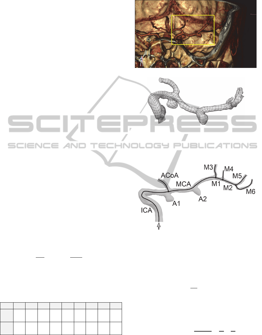
distinguishable. A direct volume visualization of a
vessel of interest is shown in figure 1(a).
The Marching-cubes algorithm (Lorensen and
Cline, 1987) was used for inner vessel surface
reconstruction as a CT haunsfield isosurface. A
resulting polygonal mesh was further converted into
a set of parametric surfaces. This is a common way
for setting a geometry for Computer-Aided Design
(CAD) systems (see fig. 1(b)).
All parts of the vessels and two aneurisms were
labelled and numbered, and the final scheme of the
investigated system is shown in figure 2. The arrow
indicates the direction of blood flow.
3 VESSEL PARAMETERS
DETECTION
For each straight vessel of the system volume
and lateral surface area
were determined.
Imagining the vessel as a cylinder with radius
and
length
and representing
and
as
,
2
,
(1)
we will get
2
,
4
.
(2)
Obtained length and radius of each vessel are listed
in table 1.
Table 1: Obtained geometric parameters (length and
radius) of the vessels.
Vessel ICA MCA M1 M2 ACoA M3 M4 M5 M6
Length
[mm]
40.5 32.6 9.48 8.8 11.5 14.1 5.09 9 11.5
Radius
[mm]
1.98 1.15 0.91 0.96 1.09 0.83 0.58 0.84 0.64
(a)
(b)
Figure 1: (a) anatomical direct volume visualization of the
described vessel system, (b) CAD geometry representation
of the system.
Figure 2: Scheme of the vessels (ICA – Internal Carotid
Artery, ACoA – Anterior Communicative Artery, MCA –
Middle Cerebral Artery) and aneurisms (A1 and A2).
Resistance of a vessel is a number that
characterizes the dependence of a pressure drop ∆
at ends of the vessel on a constant volume flow :
∆
.
(3)
The resistance of a vessel system can be calculated
similarly to the electrical circuit schemas using
formulas (4) for series and parallel connection of
vessels.
,
.
(4)
For laminar flows the resistance of a vessel does not
depend on the flow and can be calculated using
the vessel geometry and the liquid parameters.
BloodFlowPredictionandVisualizationwithintheAneurysmoftheMiddleCerebralArteryafterSurgicalTreatment
109

In our calculations two methods were tested for
resistance estimation:
Poiseuille equation;
Numerical experiment.
3.1 Poiseuille Equation
In fluid dynamics the Hagen–Poiseuille law is a
physical law that gives the pressure drop in a fluid
flowing through a long cylindrical pipe:
∆
8
,
(5)
where ∆ is the pressure drop, is the length of
pipe, is the dynamic viscosity of liquid, is the
volumetric flow rate and is the radius.
Thus, the resistance of a vessel can be calculated
using the following equation:
∆
8
.
(6)
3.2 Numerical Experiment
For the vessel resistance measurement Reynolds-
Averaged Navier-Stokes equations can be used.
A constant flow nave been simulated through
each vessel and a pressure drop was measured. The
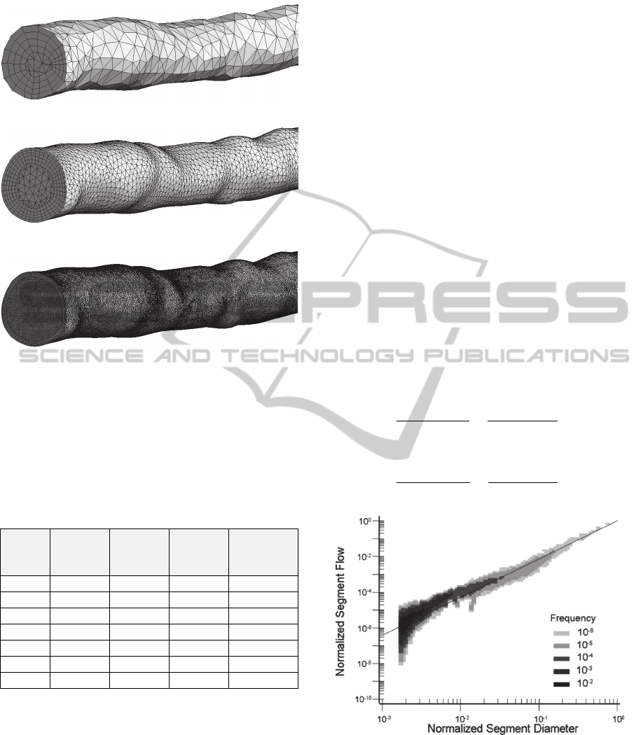
geometry of a vessel was fragmented into the mesh
of finite elements. The approximate size of elements
was selected 0.2 mm. The selection of element size
is described in the next section. The mesh is more
fine near the wall of a vessel to provide better fluid-
wall interaction (see figure 3). ANSYS CFX 15.0
was used for computation task.
The blood was set as a Nuewton liquid with
density 1080 [kg/m
3
] and viscosity
0.00388 [Pa∙s]. These parameters correspond to
normal blood parameters (Brown et al, 2013).
Volumetric flow is 10 [mm
3
/s].
Figure 3: Adjacent layer of the mesh.
The results of resistance measurement via Hagen–
Poiseuille equation and the numerical experiment
are shown in table 2.
Table 2: Resistance of the vessels measurement detected
via Hagen–Poiseuille equation (R, Poiseuille) and the
numerical experiment (R, ANSYS).
Vessel ICA MCA M1 M2 ACoA
R, Poiseuille
[Pa∙s/mm
3
]
0.026 0.187 0.138 0.103 0.081
R, ANSYS
[Pa∙s/mm
3
]
0.128 0.249 0.06 0.151 0.235
Vessel M3 M4 M5 M6
R, Poiseuille
[Pa∙s/mm
3
]
0.296 0.443 0.177 0.663
R, ANSYS
[Pa∙s/mm
3
]
0.783 1.483 0.196 1.812
4 ELEMENT SIZE SELECTION
To determine the optimal size of finite elements to
use in the computational experiments for vessel
resistance estimation real vessel geometry was used
(see fig. 4 (a)). The resistance of this vessel was
calculated using Hagen–Poiseuille Equation and
using numerical flow computation with different
element sizes.
To make the Hagen–Poiseuille equation result
more accurate the vessel was fragmented at 15 parts
(see fig. 4 (b)). Radius and length of each part were
determined and a resistance of each part was
computed. The total resistance of the vessel was
calculated as a resistance of a series connection of
several vessels.
(a)
(b)
Figure 4: (a) The geometry of the examined vessel and (b)
its fragmentation on 15 parts.
Finite element meshes with different element size
were tested. The element size was 1 mm, 0.7 mm,
0.3 mm, 0.2 mm, 0.1 mm, 0.08 mm and 0.05 mm
with total number of elements 7530, 12947, 57365,
136550, 627121, 1028359 and 2895589
respectively. Examples of some meshes are
presented in figure 5.
IMTA-52015-5thInternationalWorkshoponImageMining.TheoryandApplications
110
(a)
(b)
(c)
Figure 5: The finite elements mesh: (a) 7530 elements, (b)
57365 elements, (c) 1028359 elements.
To produce distinctly laminar flow the volumetric
flow 10 mm
3
/s was simulated.
The results of obtained resistance and
computation time are in table 3.
Table 3: Obtained resistance of the vessel.
Element
size,
[mm]
Elements
count
∆,
[Pa]
R,
[Pa∙s/mm
3
]
Computation
Time
1 7 530 1101.6 2.35 17 s
0.7 12 947 1181.96 2.53 14 s
0.3 57 365 1033 2.21 23 s
0.2 136 550 1030.12 2.2 38 s
0.1 627 121 1016.49 2.17 3 min 10 s
0.08 1 028 359 1012.82 2.17 6 min 13 s
0.05 2 895 589 1011.55 2.16 7 min 42 s
It can be seen that approximately 150 thousands
elements give an appropriate accuracy of
measurement with relatively low computation time
costs.
5 PHYSIOLOGICAL MODEL
There have been numerous theoretical attempts to
explain the design of vascular trees based on the
principles of minimum work (Murray, 1926a,b, Oka,
1974), optimal design (Rosen, 1967), minimum
blood volume (Kamiya and Togawa, 1972) and
minimum total shear force on the vessel wall (Zamir,
1976, 1977). These attempts have resulted in
relationships between the geometry and flow
parameters of the mother and daughter vessels at a
bifurcation.
Figure 6 shows the relationship between
normalized flow through a vessel segment and
normalized segment diameter for the arterial tree,
excluding the capillaries. This is an isodensity plot
showing five layers of frequency. As expected, the
majority of vessels are the smaller-diameter
arterioles. The diameter and flow are normalized
with respect to the inlet, most proximal segment.
The relationship obeys a power law relation as
suggested by Murray’s law. However, the value of
exponent is not 3, as predicted by Murray’s law. As
determined by least-squares fits of the data, the
exponent has values of 2.2, 2.1 and 2.1 for RCA,
LAD, and LCx, respectively (Mittal et al, 2005).
In our calculations we assume that volumetric
flow in daughter vessels at a bifurcation be
calculated using the following equations:
.
.
.
.
.
.
,
.
.
.
.
.
.
,
(7)
Figure 6: An isodensity plot showing 5 layers of frequency
between normalized stem flow and normalized diameter of
the stem for the left anterior descending coronary artery
(LAD) arterial tree.
where is a volumetric flow in mother vessel,
and
are flows in daughter vessels,
and
are
diameters of daughter vessels and
and
are
BloodFlowPredictionandVisualizationwithintheAneurysmoftheMiddleCerebralArteryafterSurgicalTreatment
111

cross-section areas.
The flow in the ICA was taken from tables
2.5/ 2500
/. Using (5) and the data
from table 1 the flow in all parts of investigated
vessel system has been calculated.
After the volumetric flows in all considered
vessels are determined the numerical calculation can
be performed. The pressure in ICA was set 13000
Pa. The pressure in capillaries was set 3000 Pa. The
laminar steady flow model was used.
The total pressure drop from ICA to capillaries
occurs in investigated visible vessels and in invisible
vessels (too small for CT or MRI scanning). The
resistance of invisible part of a system is a peripheral
resistance. The peripheral resistance is a crucial
value in flow prediction and can be calculated as
.
(8)
The results of volumetric flow in the vessels and
peripheral resistances calculation are in table 4. The
pressure in aneurisms A1 and A2 was determined
11104 Pa and 10230 Pa.
Table 4: A volumetric flow through the vessels; peripheral
resistances.
Vessel ICA MCA M1 M2 ACoA M3 M4 M5 M6
Q,
[mm
3
/s]
2500 1419 888 543 1081 531 345 316 227
R
peripheral
,
[Pa∙s/mm
3
]
– – – – 8.99 17.3 26.3 28.6 41.4
6 TREATMENT MODELLING
For a surgical treatment modelling we assume that
vessels M3 and M5 were clipped.
To estimate the flow
through the clipped
vessel system the total resistance
of whole system
(including visible resistances and peripheral
resistances) was computed using (4). The vessels
M3 and M5 pass zero flow, therefore the resistance
of these vessels is infinity. Knowing the resistance
the flow
can be calculated as
.
(9)
The pressure in the carotid and capillaries remains
unchanged and is 13000 Pa and 3000 Pa
respectively. The obtained value of
is 2.061/.
Since the clipped geometry cannot be considered
as physiological model the formulas (5) are
unsuitable for calculating a volumetric flow through
each separate vessel at bifurcations. Instead the
following formulas may be used:
,
,
(10)
where
and
are total resistances of vessel
branches (including visible part and peripheral
resistances).
The results of flow computation in the clipped
system are in table 5.
Table 5: Volumetric flow through the vessels after surgical
treatment and the change of the flow compared to the
initial state.
Vessel ICA MCA M1 M2 ACoA M3 M4 M5 M6
Q,
[mm
3
/s]
2061 715 715 287 1346 0 428 0 287
∆Q,
[mm
3
/s]
439 704 173 256 265 531 83 316 60
Index
[%]
82.4 50.4 80.5 52.9 124.5 0 124.1 0 126.4
Using the obtained flows a numerical modelling run
was conducted to calculate pressures in all vessels.
The pressure in aneurisms A1 and A2 after the
surgical treatment was determined 11831 Pa and
11502 Pa respectively, which is 727 Pa and 1272 Pa
higher than before treatment.
7 CONCLUSIONS
Mathematical modelling is a powerful tool for blood
flow study, prediction and visualisation. Using
camera parameters from ANSYS give possibilities
to show computational results, such as flow
velocities (see figure 7(a)), pressure (fig. 7(b)) and
wall shear stress (fig. 7(c)), over the anatomical
image of brain vessels. It makes obtained results
more clear and intuitive and enhances the quality of
surgical treatment planning.
In future work we are going to take into account
the elasticity of the vascular wall and to validate
obtained results in vitro and in clinical practice.
IMTA-52015-5thInternationalWorkshoponImageMining.TheoryandApplications
112
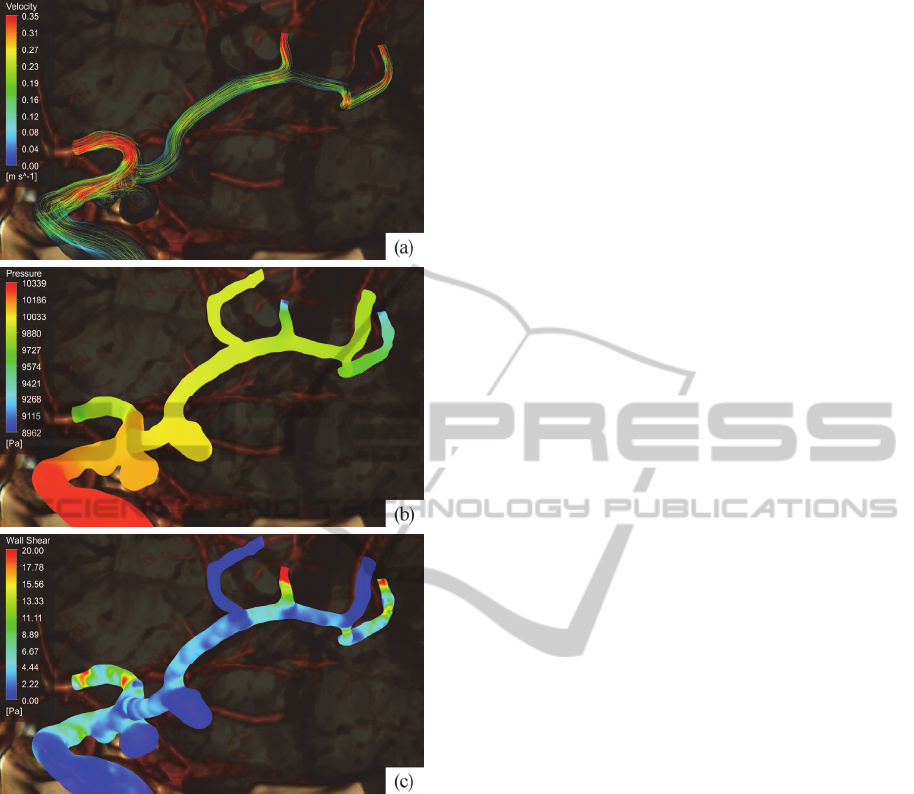
Figure 7: Visualisation of blood flow parameters: (a) flow
stream velocity, (b) blood pressure within the vessels, (c)
wall shear stress on the vessel boundary.
REFERENCES
Brown, D., Wang, J., Ho, H., Tullis, S. (2013) 'Numeric
Simulation of Fluid–Structure Interaction in the Aortic
Arch', Comp. Biomechanics for Medicine, pp. 13-23.
Cebral, J.R., Castro, M.A., Soto, O., Löhner R, Alperin N.
(2003) 'Blood-flow models of the circle of Willis from
magnetic resonance data', J. of Engineering
Mathematics, vol. 47(3-4), pp. 369–386.
Chupakhin, A.P., Cherevko, A.A. (2012) 'Measurement
and Analysis of Local Cerebral Hemodynamics in
Patients with Vascular Malformations of the Brain',
Circulation Pathology and Cardiac Surgery, vol. 4.
pp. 27–31. (in Russian).
Kamiya, A., Togawa, T. (1972) 'Optimal branching
structure of the vascular tree', Bull. Math. Biophys,
vol. 34, pp. 431–508.
Kim, H.J., Vignon-Clementel, I.E., Figueroa, C.A.,
Jansen, K.E., Taylor, C.A. (2010) 'Developing compu-
tational methods for three-dimensional finite element
simulations of coronary blood flow', Finite Elements
in Analysis and Design, vol. 46, pp. 514–525.
Krylov, V.V., Gavrilov, A.V., Prirodov, A.B., Grigoryeva,
E.V., Ganin, G.V., Arkhipov, I.V., Yatchenko, A.M.
(2013a) 'Modeling of hemodynamic changes in the
arteries and arterial brain aneurysm in vascular spasm',
Neurosurgery, vol. 4, pp. 16–25.
Krylov, V., Godkov, I. (2011a) 'Hemodynamic Factors of
Formation, Growth and Rupture of Brain Aneurysms',
J. of Neurology, vol. 1. pp. 4–9. (in Russian).
Krylov, V.V., Godkov, I.M. (2011b) 'Brain Aneurysm
Surgery', Moscow, New Time. pp. 23–35. (in Russian).
Krylov, V., Lemenev, V., Murashko, A., Luk'yanchikov,
V., Dalibaldyan V. (2013b) 'The Treatment of Patients
with Atherosclerotic Damage of Brachiocephalic
Arteries Combined with Intracranial Aneurysms', J. of
Neurosurgery, vol. 2. pp. 80–85. (in Russian).
Lorensen, W. E., Cline H.E. (1987) 'Marching Cubes: A
high resolution 3D surface construction algorithm',
Computer Graphics, vol. 21(4), pp. 163–169.
Mittal, N., Zhou, Y., Linares, C., Ung, S., Kaimovitz, B.,
Molloi, S., Kassab G.S. (2005) 'Analysis of blood flow
in the entire coronary arterial tree', Am. J. Physiol.
Heart Circ. Physiol, vol. 289, pp. H439–H446.
Murray, C.D., (1926a) 'The physiological principle of
minimum work. The vascular system and the cost of
blood volume', Natl Acad. Sci. USA 12, pp. 207–214.
Murray, C.D., (1926b) 'The physiological principle of
minimum work applied to the angle of branching of
arteries', J. Gen. Physiol, vol. 9, pp. 835–841.
Oka, S. (1974) 'Biorheology', Tokyo: Syokabo.
Olufsen, M.S., Peskin, C.S., Kim, W.Y., Pedersen, E.M.,
Nadim, A., Larsen J. (2000) 'Numerical Simulation
and Experimental Validation of Blood Flow in
Arteries with Structured-Tree Outflow Conditions',
Ann. of Biomed. Eng, vol. 28(11), pp. 1281–1299.
Rosen, R. (1967) 'Optimality Principles in Biology',
London: Butterworths.
Sforza, D.M., Putman, Ch. M., Cebral, J.R. (2009)
'Hemodynamics of Cerebral Aneurysms', Annu Rev.
Fluid Mech, vol. 4. pp. 91–107.
Tateshima, S., Tanishita, K., Omura, H., Villablanca, J.P.,
Vinuela, F. (2007) 'Intra-Aneurysmal Hemodynamics
during the Growth of an Unruptured Aneurysm: In
Vitro Study Using Longitudinal CT Angiogram
Database', Am. J. Neuroradiol.
vol. 28, pp.622–627.
Watton, P., Ventikos, Y., Holzapfel, G. (2011) 'Modelling
Cerebral Aneurysm Evolution', Stud. Mechanobiol
Tissue Eng. Biomater, vol. 7, pp. 373–399.
Zamir, M. (1976) 'The role of shear forces in arterial
branching', J. Gen. Biol. vol. 67, pp. 213–222.
Zamir, M. (1977) 'Shear forces and blood vessel radii in
the cardiovascular system', J. Gen. Physiol. vol. 69,
pp. 449–461.
BloodFlowPredictionandVisualizationwithintheAneurysmoftheMiddleCerebralArteryafterSurgicalTreatment
113
