Test of New Control Strategies for Room Temperature Control
Systems
Fully Controllable Surroundings for a Heating System with Radiators
Nina Kopmann, Rita Streblow and Dirk Müller
RWTH Aachen University, E.ON Energy Research Center, Institute for Energy Efficient Buildings and Indoor Climate,
Mathieustr. 10, 52074 Aachen, Germany
Keywords: Single Room Heating Control, Hardware-in-the-Loop, Thermostatic Valve.
Abstract: About one third of Germany’s energy demand is used for room heating thus offering a huge potential for energy
savings. The development of intelligent home energy systems should optimize the energy consumption of
buildings. In Germany the most common way to control the room temperature while heating is to use a
thermostatic valve. This temperature-control system is self-sustaining but has no possibility to communicate to the
heating system or other devices in the household. For the test and development of new control strategies and the
appropriate components a Hardware-in-the-Loop test bench for hydraulic network applications is developed at the
E.ON Energy Research Center. This test bench allows the test of a heating system of a flat in a controllable
surrounding under dynamic boundary conditions. In this paper the new test bench concept will be described.
1 INTRODUCTION
The development of home energy systems forces
more and more the investigation of new control
systems for single room heating control. In Germany
the most common way to control the temperature in a
room while heating is to use a thermostatic valve. The
user can define a set temperature and the thermostatic
valve reduces or increases the volume flow in the
radiator to adapt the heat output of the radiator. This
temperature control system is self-sustaining but has
no possibility to communicate to the heating system
or other devices in the household. New electrical
valves are designed to control the room temperature
and to communicate with the home energy system.
The use of these electrical actors is still in a
developing state, and especially new investigations
have to be tested in controllable surroundings.
This paper will show a test bench concept to develop
and test new control strategies and components for
single room heating. To combine the advantages of
static experiments with fixed boundary conditions
and the dynamic uncontrollable field studies we use a
hardware-in-the-loop (HiL) system. The HiL testing
is applied in many laboratories for the test and
development of building automation control systems
and heat supply units, as described in Barth, 2010 and
Bianchi, 2005. The special feature of the described
test bench is the reproduction of the room
environment under dynamic and controllable
surroundings.
2 CONCEPT OF THE TEST
BENCH
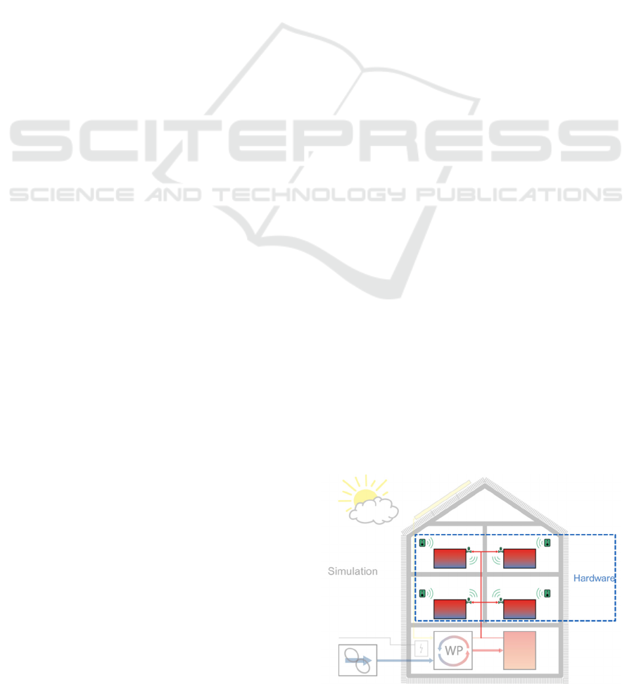
With the test bench described in this paper it is
possible to test room temperature control systems in
dynamic and controllable surroundings realized with
a HiL coupling, see Figure 1.
Figure 1: Scheme of the HiL test bench for single room
heating control systems and components.
277
Kopmann N., Streblow R. and Müller D..
Test of New Control Strategies for Room Temperature Control Systems - Fully Controllable Surroundings for a Heating System with Radiators.
DOI: 10.5220/0005478902770282
In Proceedings of the 4th International Conference on Smart Cities and Green ICT Systems (SMARTGREENS-2015), pages 277-282
ISBN: 978-989-758-105-2
Copyright
c
2015 SCITEPRESS (Science and Technology Publications, Lda.)
The real hardware (radiator, thermostatic valve,
hydraulic net and if applicable heat supply unit) will
be examined under dynamic boundary conditions,
which will be defined using a coupled simulation in
Modelica.
The test bench consists of four rooms, which are
heated with radiators. The hydraulic network is
similar as in a small flat. These four rooms are
coupled with a dynamic simulation in Modelica, so
that each room can react dynamically as it exchanges
the boundary conditions with the simulation. The type
of building and the weather can be changed in the
simulation setup. To test the direct communication
with the heat supply system, the system has the
possibility to provide the heat by an installed
condensing boiler or water/water heat pump. But
even other heat supply systems can be simulated and
the supply conditions can be emulated at the test
bench.
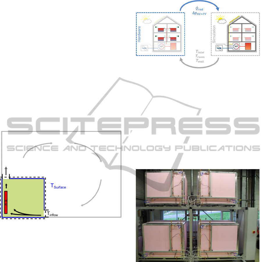
Figure 2: Reduced space requirements by downsizing the
volume of each room.
To reduce the required space for the test bench we
downsize the enclosing volume of the radiator to
about 3 to 4 m³ as shown in Figure 2. More
information about this concept can be found in
Kopmann et al., 2011. The boundary conditions
influencing the heat emission of a radiator are the
surface temperatures of the enclosing walls and the
room’s air temperature. These boundary conditions
are calculated in Modelica and relayed onto the test
bench. We use the measured heat emission of the
radiator and the pressure drop at the thermostatic
valve as boundary condition for the simulation. The
HiL concept is shown in Figure 3.
Figure 3: Data transfer using the HiL coupling.
2.1 Description of the Supply Structure
The four coupled rooms are installed in a rack
construction which allows changing the components
in each cabin individually, see Figure 4. Radiators of
type 22 with a nominal heat output of 1570 W at
70/60/20 are installed in three rooms and the fourth
room contains a radiator of type 11 with only 890 W
nominal heat output. Each room is arranged with a
standard valve body and the control component
(thermostatic valve or electrical actuator) can be
changed easily.
Figure 4: Installation of the four coupled rooms.
For the evaluation of the single room heating control
the important parameters in each cabin are measured.
The heat emission of each radiator is determined with
the inlet and outlet temperature (
,
,
,
) and the
volume flow
,
. The working process of the
installed control valve is measured by the pressure
drop
and the valve lift . And the condition of
each room can be described with the indoor air
temperature
and the defined surface and inlet air
temperatures (
,
).
SMARTGREENS2015-4thInternationalConferenceonSmartCitiesandGreenICTSystems
278
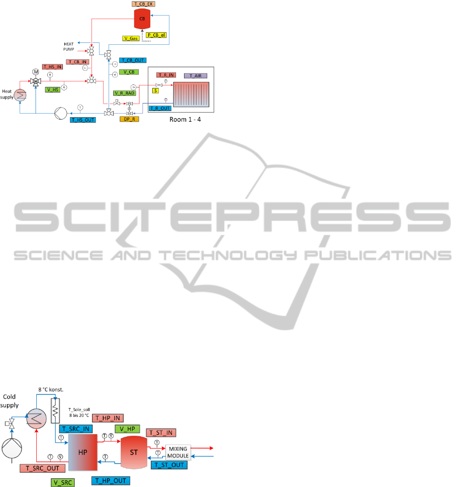
Figure 5: Installed supply structure of the test bench.
There are three possible supply units installed at the
moment. On the one hand the central heat supply of
the test hall provides the required supply temperature
,
of a simulated heat source. The control of the
supply temperature
,
is realized with a three-
way-valve in the form of a bypass control system, see
Figure 5 on the left side. The inlet and outlet
temperature (
,
,
,
) and the volume
flow
of the supply system are measured to
determine the total heat output of the system.
On the other hand an installed condensing boiler
allows the test of a real hydraulic heating network of
a small flat. For the analysis of the boiler efficiency
the gas flow
,
, the electric consumption
,
and the exhaust temperature
,
can be measured,
shown in the upper part of Figure 5. The evaluation
of the heat output of the condensing boiler is possible
by measuring the appropriate temperatures
(
,
,
,
) and the volume flow
.
Figure 6: Supply structure for the water/water heat pump
system.
For further research activities it is interesting to test
the performance of the four coupled rooms in
combination with a heat pump. Therefor the supply
structure of the test bench provides the integration of
a water/water heat pump, a storage tank and an
appropriate mixing module. The included testing
equipment, shown in Figure 6, measure the important
state values of the heat pump source
(
,
,
,
,
), the circuit between heat
pump and storage tank (
,
,
,
,
) and the
temperatures after the storage tank (
,
,
,
).
The heat pump needs a defined inlet temperature
of 8 to 20 °C, which represents the heat source. The
infrastructure of the test hall provides a constant
supply temperature of 8 °C, and the higher
temperatures are realized with a heating rod.
2.2 Definition of the Boundary
Conditions
The ambient air temperature and the simulated room
parameters (
,
) influence the heat output
and with it the air temperature
in the small scaled
room. As mentioned above these simulated
parameters need to be converted into the correct
boundary conditions for the small-scaled ambient.
In this paper we will describe the idea of the
small-scaled concept and first results regarding the
control system and the behaviour of the setup will be
shown. Further information about the conversion into
the small-scaled boundary conditions will be
published in an upcoming proceeding, as the received
results are not verified yet.
The surface temperature
is a function of
the simulated wall and room temperature, and also
dependent of the according view factors of the scaled
room parameters. These view factors are described in
Glück, 1990. The inlet air temperature
and the
volume flow are a function of the current room
temperature, which correlation is shown in Kopmann
et al., 2011. But also the ambient temperature
influences the inlet air temperature as lower ambient
temperatures results in a higher heat output and that
means larger temperature gradient of the air in a real
room.
=
,
,
)
=
,
)
In this paper we will present the characteristic of the
test bench in terms of static boundary conditions
without any room temperature control. The maximum
heat output will be examined by using low
temperature supply boundary conditions according
the surface and the inlet air temperature
(
,
). Furthermore the stability and the
repeatability of the static boundary conditions are
examined and lately the control mode of the system is
shown.
2.2.1 Heat Output of the Test Bench
The Table 1 shows the summarized heat amount of
the four coupled rooms. The presented temperatures
TestofNewControlStrategiesforRoomTemperatureControlSystems-FullyControllableSurroundingsforaHeating
SystemwithRadiators
279

are the mean values of all four rooms in the time
period considered. The influence of the supply
temperature
is shown by using three different
temperature levels 75 °C, 60 °C and 45 °C. The total
volume flow of the heating water in all three states is
constantly 6 l/min and the total air flow 440 m³/h.
Table 1: Heat output using static, low boundary conditions
at three different supply temperatures.
∑
[W]
[°C]
[°C]
[°C]
75
6215
22.9
SD=0.08K
10.1
SD=0.04K
15.7
SD=0.06K
60
4353
19.9
SD=0.05K
10.0
SD=0.03K
15.4
SD=0.02K
45
2600
17.7
SD=0.05K
9.9
SD=0.02K
15.4
SD=0.01K
A high supply temperature (
=75 °) and low
boundary conditions (
= 10 °,
=
15,0 °) result in the maximum heat output of 6.2
kW. In this case the air temperature
in the cabin
is in a warm state with 23 °C.
Lower supply temperatures result in lower heat
output and respectively lower air temperatures.
2.2.2 Stability of the Setup
To test different control strategies a stable and
controllable surrounding is important. The
measurements in Table 1 are obtained using a surface
temperature of 10 °C and an air inlet temperature of
16 °C. The surface temperature in all three states is
adjusted correctly. The air inlet temperature is about
0.4 to 0.7 K above the set-point due to an insufficient
air cooling.
The mean standard derivation (SD) in all cases of
the surface and the air inlet temperature is < 0.05 K
which means a nearly constant control. The air
temperature in the cabin has a standard derivation of
< 0.08 K, which means that the boundary conditions
are stable enough to test control algorithm in this
setup.
2.2.3 Repeatability of the Setup
For the comparison of different control strategies and
various components the repeatability of the setup is
an important fact. Therefore two analysed data of
each of the supply temperatures 75 °C and 45 °C are
displayed in Table 2. These series of measurements
were obtained using the same boundary conditions as
mentioned above.
The measured results, for the supply temperature
of 45 °C, show nearly identic results in all mentioned
data. The difference of the heat output and the air
temperature in the cabin in the two analysed series is
less than 1 %.
Table 2: Repeatability of the measured data at two supply
temperatures.
∑
[W]
[W]
[°C]
[°C]
[°C]
[°C]
75
6215
-134
2%
22,9
+0,7
3%
15,7 23,4
6081 23,6 16,8 24,3
45
2600
-11
0,4%
17,7
+0,1
0,6%
15,4 23,1
2589 17,8 15,5 23,2
The comparison of the heat output at a supply
temperature of 75 °C is also satisfactory with a
difference of 2 %. Especially when the increase of the
temperature in the test hall
of 1 K between the
two analysed series is considered.
The installed air cooling unit provides a
temperature level below the hall temperature for the
air supply temperature (
). The maximum
temperature difference between the hall temperature
and the air inlet temperature
is about 8 K
providing an air volume flow of 400 m³/h with the
installed cooling capacity. That means that the higher
ambient temperature in the second measurement
series using a supply temperature of 75 °C results in
a higher inlet temperature of the cooled air. Hence the
air temperature in the cabin
rises by 1 K and as a
consequence the heat output of the radiator decreases.
These results illustrate that the repeatability of the
measurements is dependent of the correct control of
the boundary conditions.
2.2.4 Control Mode
For the use of dynamic boundary conditions at the test
bench, it is important that the temperature control
units adapt satisfactory after the set-point is changed.
To analyse the control mode of the setup, Figure
7
shows the profile of the surface temperature (blue
lines) and the air inlet temperature (green lines) at a
set-point change. The set-point of the air inlet is
reduced from 20 °C to 16 °C and the set-point for the
surface temperature is reduced from 14.5 °C to 11.5
°C.
In the diagram we have to distinguish between the
surface temperature
and air inlet tempe-
rature
(dashed lines) and the controlled
temperatures (
,
,
) of these control units (solid
SMARTGREENS2015-4thInternationalConferenceonSmartCitiesandGreenICTSystems
280
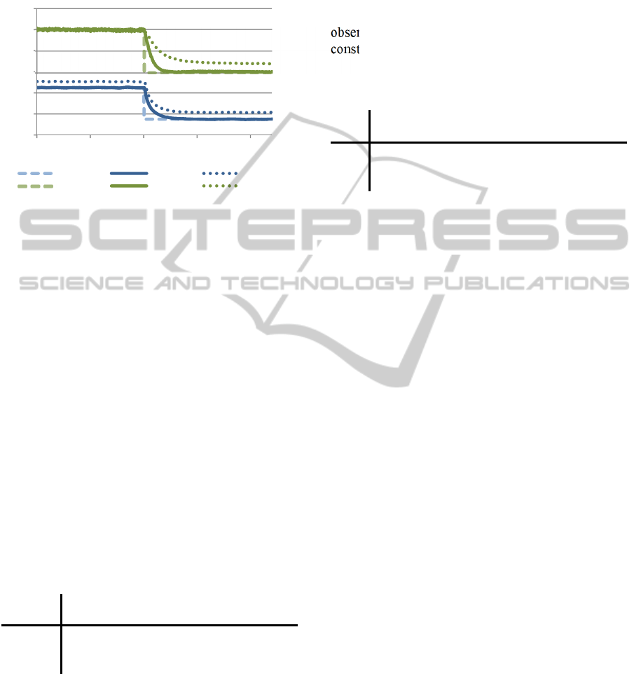
lines). The control temperatures are necessary due to
the large dead times in the control loops, which forces
an appropriate control value closer to the manipulated
variable.
Figure 7: Control response of the surface temperature and
the air inlet temperature.
The set-point of the air inlet is controlled using an
electrical heater and the controlled temperature
is
measured directly behind this heating unit. The
control needs only 15 minutes to adapt to the new set
point and has a low control deviation (
=
19.97 °) and a stable control response ( =
0.06 ), see Table 3. Behind the control unit with the
electrical heater the air flow passes a short air duct
before being inducted in the cabin. Using an inlet air
temperature of 20 °C, which is similar to the hall
temperature
, the controlled temperature
corresponds with the air inlet temperature
at the
cabins. Lower air inlet temperatures result in higher
heat losses in the air ducts so that the temperature
increases about 0.8 K before being inducted in the
cabin. A cascade control will be implemented for
further investigations to eliminate the control
deviation.
Table 3: Mean temperatures and standard deviation to
analyse the control mode of the air inlet temperature.
,
[°C]
[°C]
[K]
[°C]
[K]
air
20 19.97 0.06 19.87 0.03
16 16.02 0.02 16.84 0.04
To control the surface temperature
the inlet
temperature of the cooled walls
,
is used as the
controlled value. The control is also satisfactory, as
the set point is adapted after 20 minutes without
control deviation and a negligible standard derivation
of 0.02 K, see Figure
7
and Table 4. The actual surface
temperature
is obtained from the arithmetic
average of the inlet and the outlet temperature of the
capillary tubes which are used to provide the surface
temperatures. Compared to the controlled
temperature this surface temperature has a constant
deviation of 0.6 K, which hardly depend on the
temperature level. This constant deviation should be
observed for further investigations by using a
constant set-point adjustment.
Table 4: Mean temperatures and standard deviation to
analyse the control mode of the surface temperature.
,
[°C]
,
[°C]
,
[K]
[°C]
[K]
sur-
face
14.5 14.50 0.02 15.07 0.02
11.5 11.50 0.01 12.15 0.01
3 CONCLUSIONS
In this paper we describe the possibility to test and
develop new control strategies and components for
single room heating control under controllable and
dynamic boundary conditions. First the concept of the
new test bench is shown and the supply structure
including the monitoring technique is described. The
results of the considered measurement series give an
overview of the behaviour of the test bench setup. The
heat output of the radiators in the cabins, the stability
and the repeatability of the measurements and the
control mode of the setup were analysed. There were
obtained some aspects to improve the control for
further investigations. These aspects will be applied
in the early future and shown in a following
publication.
ACKNOWLEDGEMENTS
Grateful acknowledgement is made for financial
support by BMWi (German Federal Ministry for
Economic Affairs and Energy), promotional
reference 03ET1169C.
We also appreciate the good cooperation with our
project partners Vaillant GmbH and Fraunhofer
Institute for Solar Energy Systems.
REFERENCES
Barth, M., Fay, A., Wagner, F. Frey, G., 2010. Effizienter
Einsatz Simulationsbasierter Tests in der Entwicklung
automatisierungstechnischer Systeme. In: Tagungs-
10
12
14
16
18
20
22
11:00:00 11:30:00 12:00:00 12:30:00 13:00:00
Temperature in °C
Time
T_KT_set T_KT_in T_surface
T_HT_set T_HT T_inlet
TestofNewControlStrategiesforRoomTemperatureControlSystems-FullyControllableSurroundingsforaHeating
SystemwithRadiators
281

band Automation 2010, S. 47-50, 15-16. Juni 2010,
Baden-Baden.
Bianchi, M., Shafai, E., Geering, H. P., 2005. Comparing
New Control Concepts for Heat Pump Heating Systems
on a Test Bench with the Capability of House and Earth
Probe Emulation, Proceedings of the 8th IEA Heat
Pump Conference: Global Advances in Heat Pump
Technology, Applications and Markets, Las Vegas,
NV, June 2005.
Glück, B., 1990. Wärmeübertragung – Wärmeabgabe von
Raumheizflächen und Rohren, Verlag für Bauwesen.
Berlin, 2. Auflage.
Kopmann, N., Adolph, M., Müller, D., 2011. Entwicklung
eines Prüfstandes zur Abbildung eines hydraulischen
Heizungsnetzwerks. In: Deutsche Kälte-Klima-Tagung
2011, Aachen, 16.-18.11 2011 / Deutscher Kälte- und
Klimatechnischer Verein. Hannover : DKV, 2011. –
ISBN 978–3–932715–47–1, S. AA IV 05.
SMARTGREENS2015-4thInternationalConferenceonSmartCitiesandGreenICTSystems
282
