
3D Positioning Algorithm for Low Cost Mobile Robots
Rafael Socas, Sebasti´an Dormido, Raquel Dormido and Ernesto F´abregas
Department of Computer Science and Automatic Control, UNED, Juan del Rosal 16, 28040, Madrid, Spain
Keywords:
3D Positioning, Mobile Robots, Sensors.
Abstract:
A new 3D positioning algorithm for low cost robots is proposed. The algorithm is based on a Finite State Ma-
chine to estimate the position and orientation of the robot. The system sets dynamically the parameters of the
algorithm and makes it independent of the noise in the sensors. The algorithm has been tested for differential
wheel drive robots, however it can be used with different types of robots in a simple way. To improve the
accuracy of the system, a new reference system based on the accelerometer of the robot is presented which
reduces the accumulative error that the odometry produces.
1 INTRODUCTION
In mobile robots applications a good positioning and
orientation estimation are crucial (Borenstein and
Feng, 1995). Different techniques can be used to
solve this problem. The most common techniques
can be divided in seven categories (Borenstein et al.,
1997; Lee and Park, 2014): 1. Odometry; 2. Inertial
navigation; 3. Magnetic compasses; 4. Active bea-
con; 5. Global Positioning Systems; 6. Landmark
navigation; and 7. Model matching. At the same
time, they can be categorized into two groups based
on the position measurements: relative, (also called
dead-reckoning which includes the categories 1 and
2) and absolute (which includes the rest of the cate-
gories). Many applications usually combine two of
them, one of each group to compensate the lacks of a
single method.
The low cost robots frequently have few sensors.
They typically have wheel encoders, accelerometers
and obstacle detectors (Siegwart et al., 2011; Everett,
1995; Faisal et al., 2014). For this reason, in this kind
of platforms, the techniques that can only be applied
are Odometry and Inertial Navigation. Although both
techniques produce accumulative errors they provide
a good short-term accuracy. The odometry measures
the distance that each wheel of the robot has trav-
elled over the time. With this information, the posi-
tion and the orientation of the robot can be obtained.
On the other hand, inertial navigation uses accelerom-
eters and gyroscopes to measure the acceleration and
the rate of rotation of the robot. These measurements
have to be integrated to obtain the position and the
orientation by inertial navigation techniques. How-
ever, the cost of the gyroscopes constrains on the en-
vironments in which they are practical for use. In low
cost robot the techniques that can be used to estimate
the position are odometry and inertial navigation with
accelerometers. In general way, low cost accelerome-
ters have poor signal to noise ratio when the robot has
small accelerations (common situation in many appli-
cations, for example in robots with constant speed),
for this reason, the positioning and orientation esti-
mation by accelerometers in low cost platforms is a
bad solution (Liu and Pang, 2001). On the other hand,
the accelerometers have a good performance in tilt an-
gles estimation (Trimpe and D’Andrea, 2010; Luczak
et al., 2006).
In this paper a new 3D positioning algorithm for
for low cost robots is proposed, it combines odometry
and tilt estimation to obtain the position and the orien-
tation in 3D. Also, the tilt estimation is used as a ref-
erence system to reduce the orientation error that the
classical odometry produces. The paper is organized
as follows. Section 2 presents the 3D positioning in
mobile robots applications. The proposed algorithm
is presented in section 3. The experimental results are
analysed in section 4. And finally, the conclusions
and future work are presented in section 5.
2 3D POSITIONING AND
ORIENTATION
The estimation of the position and orientation of mo-
bile robots is one of the basic preconditions for their
5
Socas R., Dormido S., Dormido R. and Fabregas E..
3D Positioning Algorithm for Low Cost Mobile Robots.
DOI: 10.5220/0005480900050014
In Proceedings of the 12th International Conference on Informatics in Control, Automation and Robotics (ICINCO-2015), pages 5-14
ISBN: 978-989-758-123-6
Copyright
c
2015 SCITEPRESS (Science and Technology Publications, Lda.)
autonomy. The aim of this work is to estimate the
position and orientation of the robot in 3D. Both es-
timations can be defined as a vector with six com-
ponents po = { ˆx, ˆy, ˆz,
ˆ
ϕ,
ˆ
θ,
ˆ
ψ} (Roberson and Schwer-
tassek, 1988). The position ( ˆx, ˆy, ˆz) and the orientation
(
ˆ
ϕ,
ˆ
θ,
ˆ
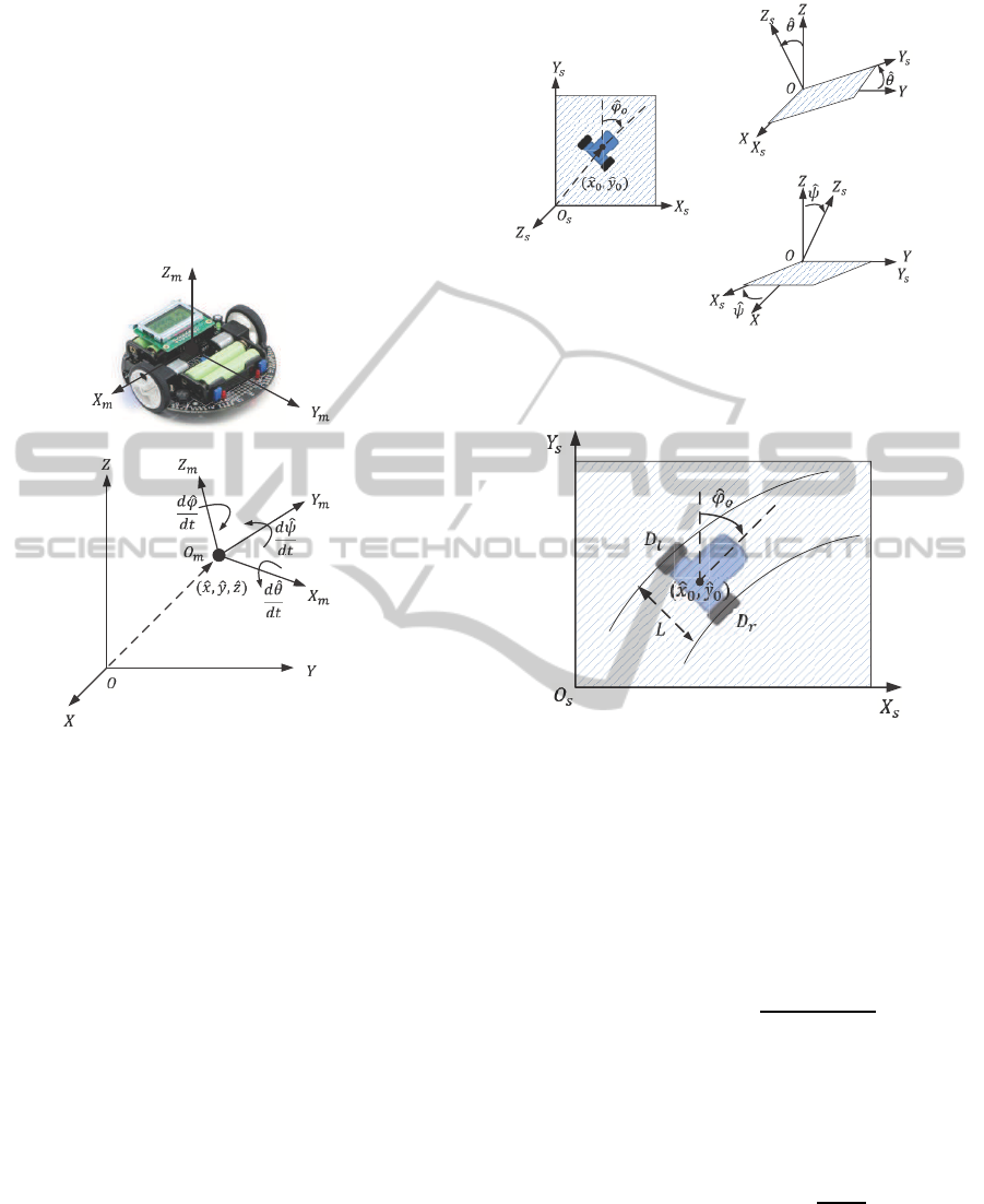
ψ) are defined with respect to the world frame
(O) as it is shown in Figure 1. The elevation
ˆ
θ, the
bank
ˆ
ψ and the heading
ˆ
ϕ are the Tait-Bryan angles.
Finally, on the robot, the moving frame (O
m
) is de-
fined.
Moving
Frame
World Frame
Moving
Frame
Figure 1: Position (ˆx, ˆy, ˆz) and orientation (
ˆ
ϕ,
ˆ
θ,
ˆ
ψ) with re-
spect to the world frame (O).
When the robot is travelling on a flat surface S,
a new reference frame can be defined O
s
(surface
frame). Via odometry the position (ˆx
o
, ˆy
o
) and the ori-
entation
ˆ
ϕ
o
with respect to the surface frame can be
calculated. A tilt estimation based on an accelerom-
eter is used to obtain the elevation
ˆ
θ and the bank
ˆ
ψ
angles of the surface S with respect to the world frame
(see Figure 2).
With the parameters ˆx
o
, ˆy
o
,
ˆ
ϕ
o
,
ˆ
θ and
ˆ
ψ the com-
ponents of the vector po can be calculated. The
methodology to estimate it will be explained in the
following sections.
2.1 Position and Orientation Estimation
via Odometry
Two differential wheels robots are the most common
low cost mobile robots. These systems usually have
wheel encoders, an accelerometer and other sensors
to avoid obstacles. When the robot is travelling on
a flat surface its position and orientation can be esti-
mated using odometry (Abbas et al., 2006; Jha and
S
S
S
a)a)
b)
c)
Figure 2: a) Position (ˆx
o
, ˆy
o
) and orientation (
ˆ
ϕ
o
) with re-
spect to the surface frame (O
s
). b) Elevation angle (
ˆ
θ). c)
Bank angle (
ˆ
ψ).
S
Figure 3: Position (ˆx
o
, ˆy
o
) and orientation (
ˆ
ϕ
o
) with respect
to the surface frame (O
s
).
Kumar, 2014). Wheel encoders allow to measure the
distances that each wheel has travelled (D
l
for the left
wheel and D
r
for the right wheel). With D
l
, D
r
and
the distance between the two wheels L (see Figure 3),
the position and the orientation of the robot can be
calculated in discrete-time using equations(1)-(3).
ˆ
ϕ
o
[n] =
ˆ
ϕ
o
[n− 1] +
D
l
[n] − D
r
[n]
L
(1)
ˆx
o
[n] = ˆx
o
[n− 1] + D
c
∗ sin(
ˆ
ϕ
o
[n]) (2)
ˆy
o
[n] = ˆy
o
[n− 1] + D
c
∗ cos(
ˆ
ϕ
o
[n]) (3)
where
D
l
: Distance travelled by left wheel.
D
r
: Distance travelled by right wheel.
D
c
: Mean distance defined by D
c
=
D
l
+D
r
2
.
L: Distance between the two wheels.
2.2 Tilt Estimation
The accelerometer is sensitive to the total accelera-
tion of the mobile robot. It is composed of the inertial
ICINCO2015-12thInternationalConferenceonInformaticsinControl,AutomationandRobotics
6
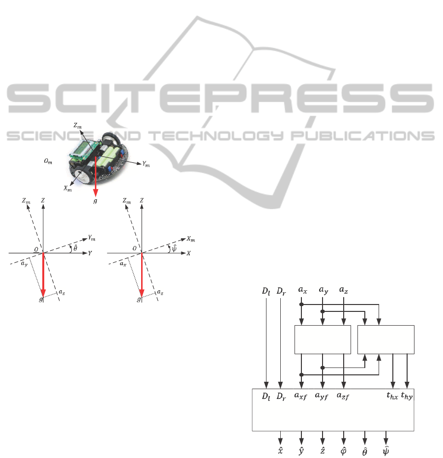
acceleration, the gravity field g, the centripetal and
the tangential acceleration. This sensor measures the
three components (a
x
,a
y
,a
z
) of the total acceleration
with respect to the moving frame (O
m
). In the two dif-
ferential wheel drive robots considered in this paper,
the gravity field is the most important component of
the acceleration, for this reason, the rest of them are
not considered.
On the other hand, the robot is made to drive three
possible rotations: the elevation
ˆ
θ, the bank
ˆ
ψ and the
heading
ˆ
ϕ angles with respect to the world frame (O).
With this assumption, the sensor in the robot is mea-
suring the gravity field g (because the movements of
the robot do not produce other accelerations or they
are irrelevant) with respect to the moving frame on
the robot (see Figure 4). In the world frame the ac-
celeration is always the same (0,0,−g) where, on the
other hand, the relationship between the accelerations
in the two frames and the rotation angles is defined by
(4).
Moving
Frame
a)
b) c)
Figure 4: a) Gravity field with respect to the moving frame,
the components (a
x
,a
y
,a
z
) are the measurements of the ac-
celerometer. b) Robot with elevation angle
ˆ
θ. c) Robot with
a bank angle
ˆ
ψ.
a
x
a
y
a
z
= R(
ˆ
θ,
ˆ
ψ,
ˆ
ϕ) ∗
0
0
−g
(4)
The rotation matrix R(
ˆ
θ,
ˆ
ψ,
ˆ
ϕ) depends on the or-
der of rotations. Therefore to calculate the angles
ˆ
θ,
ˆ
ψ and
ˆ
ϕ it is necessary to know the order of rotation.
Considering a robot that rotates first an angle
ˆ
θ and
then an angle
ˆ
ψ, the measurements in the accelerom-
eter are described by (5).
a
x
a
y
a
z
=
−g∗ cos(θ) ∗ sin(ψ)
−g∗ sin(θ)
−g∗ cos(θ) ∗ cos(ψ)
(5)
If the robot rotates first an angle
ˆ
ψ and then an angle
ˆ
θ, the accelerometer measurements are given by (6).
a
x
a
y
a
z
=
−g∗ sin(ψ)
−g∗ cos(ψ) ∗ sin(θ)
−g∗ cos(ψ) ∗ cos(θ)
(6)
Comparing (5) and (6) the components a
x
and a
y
are
different in each equation, and therefore, we can con-
clude that the problem is undetermined. If the robot
has gyroscopes, the order of rotations can be esti-
mated and consequently the rotation angles can be
calculated. As we mentioned before, low cost robots
frequently have an accelerometer but they do not have
gyroscopes. For this reason, in a general way in this
kind of robots the elevation
ˆ
θ and the bank
ˆ
ψ angle
can not be estimated.
3 ALGORITHM ARCHITECTURE
The limitations of the low cost robots to estimate the
elevation and the bank angles has been analysed in
Section 2. To avoid these problems in this paper we
assume that:
a) The two-wheel differential robot can travel only
on a flat surface and,
b) this surface might have an elevation angle or a
bank angle, but not both angles at the same time.
With the previous assumptions, to estimate the po-
sitioning in 3D and the orientation of the robot, the
discrete-time architecture depicted in Figure 5 has
been proposed.
Wheel
Encoders
Accelerometer
Low Pass
Filter
Finite State Machine
Threshold
Calculator
Figure 5: Algorithm architecture.
As it is shown in the Figure 5, the algorithm is
composed of the following signals and blocks:
3DPositioningAlgorithmforLowCostMobileRobots
7

a) Input signals, D
l
[n] and D
r
[n] directly reading
from wheel encoders, and a
x
[n], a
y
[n] and a
z
[n] from
the accelerometer.
b) A low pass filter to remove the noise in the sen-
sor’s signal. The outputs of this blocks are a
xf
[n],
a
yf
[n] and a
zf
[n].
c) A threshold calculator which obtains the thresh-
old values (t
hx
[n] and t
hy
[n]), these values will be
used in the Finite State Machine (FSM) to define the
changes between states.
d) The FSM which estimates the position and ori-
entation parameters.
e) And finally, the output signals
(ˆx[n], ˆy[n], ˆz[n],
ˆ
ϕ[n],
ˆ
θ[n],
ˆ
ψ[n]).
3.1 Low Pass Filter
Low pass filtering of the signals from the accelerom-
eter is a good way to remove the noise (both mechan-
ical and electrical) (Seifert and Camacho, 2007). In
this work, an IIR filter has been proposed (7).
a
if
[n] = (1 − α) ∗ a
i
[n] + α∗ a
if
[n− 1] (7)
for i = {x,y,z}
The inputs are the accelerometer’s signal
(a
x
[n],a
y
[n],a
z
[n]) and the outputs are the filtered
signals (a
xf
[n],a
yf
[n],a
zf
[n]). The parameter α sets
the cut off frequency and the group delay of the filter.
In the design process, α has to be selected to obtain
a good balance between the noise reduction and the
delay in the acceleration measurements.
3.2 Threshold Calculator
As we mention before, the positioning algorithm is
based on a Finite State Machine. The states, as they
will be explained in the next section, depend on the
values of the elevation angle
ˆ
θ[n] and the bank angle
ˆ
ψ[n]. When the robot is on a surface with
ˆ
θ[n] ≈ 0 or
ˆ
ψ[n] ≈ 0, the noise in the accelerometer sensor could
produce changes between states and the system could
be unstable. For this reason, the algorithm needs a
threshold system to control the changes between the
states taking in account the noise in the sensors.
As we will explain later, when the elevation and
the bank angle are close to zero (
ˆ
θ ≈ 0,
ˆ
ψ ≈ 0), the
values of the accelerations a
xf
[n] and a
xf
[n] should be
zero except by the noise in the sensor. For this reason,
the noise in these measurements will be considered in
the threshold calculator.
The noise n
x
[n] and n
y
[n] in the acceleration sig-
nals a
x
[n] and a
y
[n] can be estimated by the difference
between the acceleration signals and their filtered sig-
nals as shown in (8) and (9).
n
x
[n] = a
x
[n] − a
xf
[n] (8)
n
y
[n] = a
y
[n] − a
yf
[n] (9)
Then a simple moving averagehas been used to obtain
a stable value of the noise, then the function atan() is
applied to calculate the threshold angles by (10) and
(11).
t
hx
[n] = atan
1
l
l
∑
k=1
abs(n
x
[k])
!
(10)
t
hy
[n] = atan
1
l
l
∑
k=1
abs(n
y
[k])
!
(11)
In this way the proposed system obtains two dynamic
threshold values (t
hx
[n] and t
hy
[n]) one for each accel-
eration signal. Moreover, it has a degree of freedom,
the parameter l, which will be set depending on how
the level of noise changes over the time.
The proposed threshold calculator is depicted in
Figure 6.
…..
…..
…..
…..
Figure 6: Threshold calculator. The threshold values are
obtained as a moving average of the noise in the sensor.
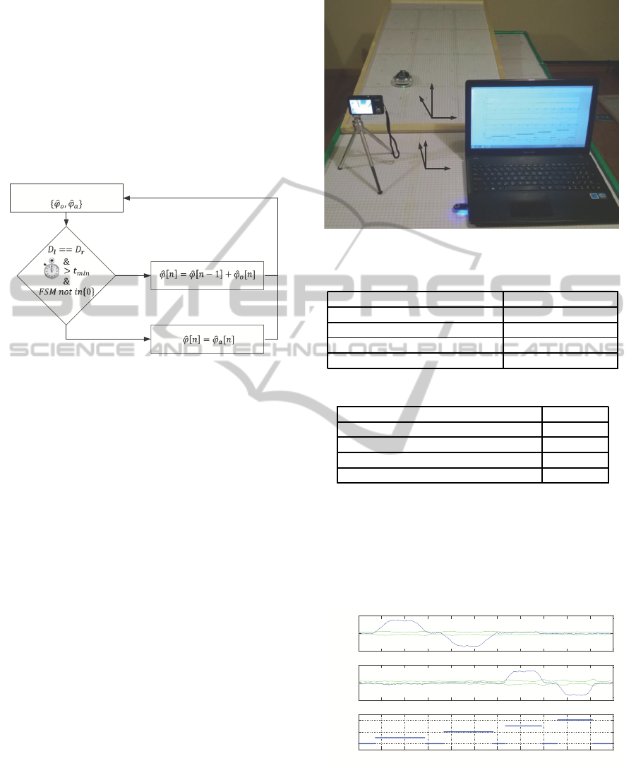
3.3 Finite State Machine
A Finite State Machine (FSM) has been included in
the architecture to estimate the position in 3D of the
robot (see Fig. 5). The inputs are the wheel en-
coders, the filtered accelerations and the threshold
values. The outputs are the estimation of the position
( ˆx[n], ˆy[n], ˆz[n]) and the orientation (
ˆ
ϕ[n],
ˆ
θ[n],
ˆ
ψ[n]) of
the robot. As we mentioned before, the robot only can
travel on a flat surface and this surface could have an
elevation angle or a bank angle with respect to the
world frame, but it can not have two rotations at the
same time. Taking into account these considerations,
in this section the behaviour of the FSM have been
developed.
As it is shown in the Figure 7, the FSM has
five states and five conditions to change between the
ICINCO2015-12thInternationalConferenceonInformaticsinControl,AutomationandRobotics
8

Rotation X+
Rotation X-
Rotation Y+
Rotation Y-
(State 0)
(State 1)
(State 2)
(State 3) (State 4)
Start
Figure 7: The FSM has five states (State 0, 1,2,3,4 and 5)
and five transition conditions (C
0
,C
1
,C
2
,C
3
and C
4
).
states. The meaning of each state is presented in the
following definitions:
a) State 0: The robot is on a surface without ele-
vation angle (
ˆ
θ ≈ 0) and without bank angle (
ˆ
ψ ≈ 0)
with respect to the world frame.
b) State 1: The robot is on a surface with a positive
elevation angle (
ˆ
θ > 0) and without bank angle (
ˆ
ψ ≈
0).
c) State 2: The robot is on a surface with a neg-
ative elevation angle (
ˆ
θ < 0) and without bank angle
(
ˆ
ψ ≈ 0).
d) State 3: The robot is on a surface with a positive
bank angle (
ˆ
ψ > 0) and without elevation angle (
ˆ
θ ≈
0).
e) State 4: The robot is on a surface with a nega-
tive bank angle (
ˆ
ψ < 0) and without elevation angle
(
ˆ
θ ≈ 0).
On the other hand, we assume that the system
works in discrete-time, in each sample time the mea-
surements of the sensor (D
l
[n], D
r
[n], a
xf
[n], a
yf
[n],
a
zf
[n]) are available.
The conditions (C
0
,C
1
,C
2
,C
3
,C
4
) which control
the changes between states are defined as function
of the components of the acceleration (a
xf
[n], a
yf
[n],
a
zf
[n]), the threshold values (t
hx
[n] and t
hy
[n]) and two
positive guard parameters (H and h) as it is presented
in the following equations (12)-(18):
θ
tilt
= atan(a
yf
[n]/a
zf
[n]) (12)
ψ
tilt
= atan(a
xf
[n]/a
zf
[n]) (13)
C
0
: (abs(θ
tilt
) ≤ t
hy
[n] + h)
&(abs(ψ
tilt
) ≤ t
hx
[n] + h)
(14)
C
1
: θ
tilt
> t
hy
[n] + H (15)
C
2
: θ
tilt
< −t
hy
[n] − H (16)
C
3
: ψ
tilt
> t
hx
[n] + H (17)
C
4
: ψ
tilt
< −t
hx
[n] − H (18)
The parameters H and h create two guard bands
around the threshold values. These guards bands
make a new threshold value (t
hy
[n] + H or t
hx
[n] + H)
when the elevation and bank angles increase and an-
other one (t
hy
[n] + h or t
hx
[n] + h) when they decrease.
This method avoids instabilities when θ
tilt
≈ t
hy
or
ψ
tilt
≈ t
hx
. These parameters have to be set taking
in account the level of noise in the sensor.
3.4 Position and Orientation Estimation
In each state of the FSM an estimation of the 3D po-
sitioning has to be calculated. In the state 0 the clas-
sical odometry has been applied. For the rest of the
states a combination of tilt estimation and odometry
have been used. The aim of the 3D positioning esti-
mation is to calculate the position vector of the robot
(po[n] = { ˆx[n], ˆy[n], ˆz[n],
ˆ
ϕ[n],
ˆ
θ[n],
ˆ
ψ[n]}). Depending
on the state where the robot is, different equations
have to be applied. In the following sections, these
equations will be defined.
3.4.1 Estimation in State 0
In state 0, due to the tilt is zero, the classical odometry
has to applied as it is presented in (19)-(24).
ˆ
ϕ[n] =
ˆ
ϕ[n− 1] +
ˆ
ϕ
o
[n] (19)
ˆx[n] = ˆx[n− 1] + D
c
[n] ∗ sin(
ˆ
ϕ[n]) (20)
ˆy[n] = ˆy[n− 1] + D
c
[n] ∗ cos(
ˆ
ϕ[n]) (21)
ˆz[n] = ˆz[n− 1] (22)
ˆ
θ[n] = 0 (23)
ˆ
ψ[n] = 0 (24)
where
ˆ
ϕ
o
[n]: Heading estimation by odometry
D
l
[n]−D
r
[n]
L
D
c
[n]: Mean distance D
c
[n] =
D
l
[n]+D
r
[n]
2
.
L: Distance between the two wheels.
3.4.2 Estimation in State 1 and 2
The elevation angle
ˆ
θ[n] can be calculated in state 1
by (25) and in state 2 by (26).
ˆ
θ[n] = atan
p
a
xf
[n]
2
+ a
yf
[n]
2
−a
zf
[n]
!
(25)
ˆ
θ[n] = atan
p
a
xf
[n]
2
+ a
yf
[n]
2
a
zf
[n]
!
(26)
In both states the components
ˆ
ϕ[n], ˆx[n], ˆy[n] and
ˆ
ψ[n] have the same expressions (27) - (30)
ˆ
ϕ[n] =
ˆ
ϕ[n− 1] +
ˆ
ϕ
o
[n] (27)
3DPositioningAlgorithmforLowCostMobileRobots
9

ˆx[n] = ˆx[n− 1] + D
c
[n] ∗ sin(
ˆ
ϕ[n]) (28)
ˆy[n] = ˆy[n− 1] + D
c
[n] ∗ cos(
ˆ
ϕ[n])∗ cos(θ
a
) (29)
ˆ
ψ[n] = 0 (30)
Where θ
a
= abs(
ˆ
θ[n])
The component ˆz[n] can be calculated in state 1 by
(31) and in state 2 by (32).
ˆz[n] = ˆz[n− 1] + D
c
[n] ∗ sin(
ˆ
ϕ[n])∗ sin(θ
a
) (31)
ˆz[n] = ˆz[n− 1] − D
c
[n] ∗ sin(
ˆ
ϕ[n])∗ sin(θ
a
) (32)
3.4.3 Estimation in State 3 and 4
On the other hand, the bank angle
ˆ
ψ[n] can be calcu-
lated in state 3 by (33) and in state 4 by (34).
ˆ
ψ[n] = atan
p
a
xf
[n]
2
+ a
yf
[n]
2
−a
zf
[n]
!
(33)
ˆ
ψ[n] = atan
p
a
xf
[n]
2
+ a
yf
[n]
2
a
zf
[n]
!
(34)
In both states the components
ˆ
ϕ[n], ˆx[n], ˆy[n] and
ˆ
θ[n] have the same expressions (35) - (38)
ˆ
ϕ[n] =
ˆ
ϕ[n− 1] +
ˆ
ϕ
o
[n] (35)
ˆx[n] = ˆx[n − 1] + D
c
[n] ∗ sin(
ˆ
ϕ[n])∗ cos(ψ
a
) (36)
ˆy[n] = ˆy[n− 1] + D
c
[n] ∗ cos(
ˆ
ϕ[n]) (37)
ˆ
θ[n] = 0 (38)
Where ψ
a
= abs(
ˆ
ψ[n])
Finally, the component ˆz[n] can be calculated in
state 3 by (39) and in state 4 by (40).
ˆz[n] = ˆz[n− 1] + D
c
[n] ∗ sin(
ˆ
ϕ[n])∗ sin(ψ
a
) (39)
ˆz[n] = ˆz[n− 1] − D
c
[n] ∗ sin(
ˆ
ϕ[n])∗ sin(ψ
a
) (40)
3.5 Heading Reference System based on
Tilt Angle
The heading angle
ˆ
ϕ[n] is the most important of the
navigation parameters in terms of its influence on ac-
cumulated errors. In the proposed system, when the
robot is in the state 0 the only way to calculate this pa-
rameter is by odometry (
ˆ
ϕ[n] =
ˆ
ϕ[n−1]+
ˆ
ϕ
o
[n] where
ˆ
ϕ
o
[n] =
D
l
[n]−D
r
[n]
L
). But, when the robot is moving
on a surface with an elevation angle
ˆ
θ[n] 6= 0 or with
a bank angle
ˆ
ψ[n] 6= 0 (states 1, 2, 3 or 4), the values
of a
xf
[n] and a
yf
[n] can also be used to estimate the
heading angle of the robot.
When the FSM is in state 1, 2, 3 or 4, two estima-
tions of the heading can be obtained, one of them via
odometry
ˆ
ϕ
o
[n] and another one from the accelerom-
eter
ˆ
ϕ
a
[n] by the following equations (41)-(44).
In state 1,
ˆ
ϕ
a
[n] =
atan
|a
xf
|
|a
yf
|
if (a
xf
>0)&(a
yf
≤0)
π
2
+ atan
|a
yf
|
|a
xf
|
if (a
xf
>0)&(a
yf
>0)
π+ atan
|a
xf
|
|a
yf
|
if (a
xf
≤0)&(a
yf
>0)
3π
2
+ atan
|a
yf
|
|a
xf
|
if (a
xf
≤0)&(a
yf
≤0)
(41)
in state 2,
ˆ
ϕ
a
[n] =
π+ atan
|a
xf
|
|a
yf
|
if (a
xf
>0)&(a
yf
≤0)
3π
2
+ atan
|a
yf
|
|a
xf
|
if (a
xf
>0)&(a
yf
>0)
atan
|a
xf
|
|a
yf
|
if (a
xf
≤0)&(a
yf
>0)
π
2
+ atan
|a
yf
|
|a
xf
|
if (a
xf
≤0)&(a
yf
≤0)
(42)
in state 3,
ˆ
ϕ
a
[n] =
π
2
+ atan
|a
xf
|
|a
yf
|
if (a
xf
>0)&(a
yf
≤0)
π+ atan
|a
yf
|
|a
xf
|
if (a
xf
>0)&(a
yf
>0)
3π
2
+ atan
|a
xf
|
|a
yf
|
if (a
xf
≤0)&(a
yf
>0)
atan
|a
yf
|
|a
xf
|
if (a
xf
≤0)&(a
yf
≤0)
(43)
and finally, in state 4
ˆ
ϕ
a
[n] =
3π
2
+ atan
|a
xf
|
|a
yf
|
if (a
xf
>0)&(a
yf
≤0)
atan
|a
yf
|
|a
xf
|
if (a
xf
>0)&(a
yf
>0)
π
2
+ atan
|a
xf
|
|a
yf
|
if (a
xf
≤0)&(a
yf
>0)
π+ atan
|a
yf
|
|a
xf
|
if (a
xf
≤0)&(a
yf
≤0)
(44)
where a
xf
= a
xf
[n] and a
yf
= a
yf
[n]
Here, it is important to note that the heading es-
timation from the accelerometer
ˆ
ϕ
a
[n] is an absolute
measure of the heading angle and it does not depend
on the previous values. For this reason, this measure
is a good way to avoid the accumulated errors that the
classical odometry produces.
On the other hand, due to the acceleration signals
have to be filtered to eliminate the noise in the sen-
sor, the measurements of the acceleration have a de-
lay which depends on the parameter α of the filter (see
equation 7). In this case, if the heading estimation is
calculated as
ˆ
ϕ[n] =
ˆ
ϕ
a
[n] it would be a bad approxi-
mation, for example, when the robot is making a cir-
cular path. Nevertheless, a little time after the robot
starts to travel in straight line, the accelerations are
stable (because the values of a
xf
[n],a
yf
[n] and a
zf
[n]
do not change) and the delay does not affect.
ICINCO2015-12thInternationalConferenceonInformaticsinControl,AutomationandRobotics
10
Taking in account the previous considerations,
when the robot is travelling in straight line (D
l
= D
r
)
after certain time (time > t
min
) and the FSM is in
state 1, 2, 3 or 4, the heading estimation from the ac-
celerometer
ˆ
ϕ
a
[n] can be used as a reference value for
the heading angle. In this way, the accumulated error
that the classical odometry produces in the heading
angle can be avoided. The t
min
value has to be defined
as a function of the parameter α of the filter. The ref-
erence system proposed in this paper is depicted in
Figure 8.
Heading Estimation
yes
no
Figure 8: Proposed heading reference system.
4 EXPERIMENTAL RESULTS
To check the proposed algorithm in this paper, the
low cost mOway differential wheel drive robot has
been used. This robot has wheel encoders and a
three-axis MMA7455L accelerometer from Freescale
Semiconductor. The accelerometer has a dynamic
range from −2g to 2g (where g value is 9.81m/s
2
)
in the three axis. The positioning algorithm has been
implemented in C++ language, the algorithm runs in
a laptop with Windows OS. A radio frequency link of
2.4 GHz has been used to communicate the robot and
the laptop. A flat surface without tilt angle has been
used as the world frame and a moving surface as sur-
face frame (see section 2). Finally, a video camera
has been used to capture the real path of the robot.
The test laboratory is depicted in Figure 9.
Before checking the algorithm, the sensor and
other parameters of the robot were calibrated. The re-
sults of these procedures are presented in the Table1.
On the other hand, the parameters of the algorithm
were set as it is shown in Table 2.
Next sections, show some experiments to analyse
the response of the algorithm.
4.1 Behaviour of the FSM
To check the behaviour of the FSM, the robot was
put on the moving surface (surface frame) with a con-
Surface Frame
World Frame
mOway
Robot
PC conneted via
RF to the robot
Video
camera
Figure 9: Test laboratory.
Table 1: Robot parameters.
Sampling period t
s
= 0.2s
Distance between two wheels L = 6.6cm
Bias X acceleration a
xbias
= −0.1059g
Bias Y acceleration a
ybias
= −0.3480g
Bias Z acceleration a
zbias
= 0.0927g
Table 2: Algorithm parameters.
Filter constant α = 0.9
Length of threshold calculator l = 20
Guard value H H = 0.2
◦
Guard value h h = 0.1
◦
Minimum time in reference system t
min
= 1s
stant speed of 10.3cm/s in straight line. Then differ-
ent tilts (
ˆ
θ and
ˆ
ψ) were applied and the states of the
FSM were analysed. The elevation angle was modi-
fied from −8
◦
to 8
◦
, in the same way, the bank angle
was varied from −7.5
◦
to 7.5
◦
. The result of the ex-
periment is depicted in the Figure 10.
0 20 40 60 80 100 120 140 160 180 200 220
-10
0
10
0 20 40 60 80 100 120 140 160 180 200 220
-10
0
10
0 20 40 60 80 100 120 140 160 180 200 220
0
2
4
a)
b)
c)
Figure 10: FSM’s behaviour. a) Elevation angle in blue and
t
hy
in green. b) Bank angle in blue and t
hx
in green. c) States
of the FSM.
As Figure 10 shows, the behaviourof the system is
according to the tilt angle. When tilt angles are close
to zero, the system is in the state 0. The FSM is in
3DPositioningAlgorithmforLowCostMobileRobots
11
the state 1 or 2 depending on the value of θ
tilt
as it is
presented in Figure 10 a) and 10 c). And finally, states
3 and 4 depend on the value of ψ
tilt
as it is shown in
Figure 10 b) and 10 c).
It is important to note that the system can change
between states with an error smaller than 1
◦
in the tilt
estimation as it is presented in Figure 10.
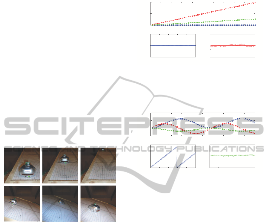
4.2 3D Positioning Estimation
Once the FSM is analysed, the next step is to check
the 3D positioning. To this end two experiments
were performed. In the first one, the robot travels in
straight line with a speed of 10.3cm/s on a surface
with a elevation angle of fifteen degrees (θ = 15
◦
).
In the second one, the robot drives a circular path
(speed of left wheel= 17.5cm/s and speed of right
wheel= 10.3cm/s) on a surface with bank angle of
minus twenty degrees (ψ = −20
◦
). The experiments
take 10 seconds in both cases. In Figure 11 some
snapshots of theses experiments are presented.
a)
b)
t=0s
t=0s
t=2s
t=10s
t=1,5s t=5s
Figure 11: Experiments for checking the 3D positioning es-
timation. a) Straight line with θ = 15
◦
and ψ = 0
◦
(state 1).
b) Circular path with θ = 0
◦
and ψ = −20
◦
(state 4).
To check the accuracy of the algorithm, the real
position (x,y,z) and orientation (ϕ,θ,ψ) of the robot
is obtained from the images of the video camera. The
estimated parameters ( ˆx, ˆy, ˆz,
ˆ
ϕ,
ˆ
θ,
ˆ
ψ) are calculated by
the proposed algorithm. The results of the first exper-
iment is depicted in Figure 12 and in Figure 13 for the
second one. As it is shown in the Figures 12 and 13
the algorithm is a good 3D positioning estimator with
a low estimation error. The elevation and the bank an-
gles do not have accumulative errors because they are
obtained directly from the accelerometer. The rest of
the parameters, will have accumulative error over the
time because they are calculated by odometry.
4.3 The Heading Reference System
To analyse how the heading reference system im-
proves the 3D positioning estimation, a new exper-
0 1 2 3 4 5 6 7 8 9 10
0
50
100
0 2 4 6 8 10
-1
0
1
0 2 4 6 8 10
0
10
20
30
a)
b)
c)
Figure 12: 3D positioning estimation in a straight line. a)
Figure 12: 3D positioning estimation in a straight line. a)
Real position (x,y,z) (solid lines) and estimated position
( ˆx, ˆy, ˆz) (square line). b) Real heading ϕ (solid line) and
estimated heading
ˆ
ϕ (circle line). c) Real elevation θ (solid
line) and estimated elevation
ˆ
θ (circle line). The bank angle
ˆ
ψ is not depicted because is zero as it was defined in (30).
0 1 2 3 4 5 6 7 8 9 10
-20
0
20
40
0 2 4 6 8 10
0
200
400
0 2 4 6 8 10
-40
-20
0
a)
b)
c)
Figure 13: 3D positioning estimation in a circular path. a)
Real position (x,y,z) (solid lines) and estimated position
( ˆx, ˆy, ˆz) (square line). b) Real heading ϕ (solid line) and es-
timated heading
ˆ
ϕ (circle line). c) Real bank ψ (solid line)
and estimated bank
ˆ
ψ (circle line). The elevation angle
ˆ
θ is
not shown due to is zero according to (38).
iment has been set up. In this case, the robot has
been programmed with a trajectory as it is shown in
the Figure 14. The real path of the robot has been
recorded by the video camera and two estimations
have been calculated in the same experiment. One
of them without the heading reference system and the
another one using this system. The real heading and
its estimations by the algorithm are presented in the
Figure 15. As it can be noticed from this figure, the
error in the heading estimation without the reference
system increases over time. However when the ref-
erence system is activated, the error in the heading
estimation does not increase.
Considering the position parameters, the results of
the experiment are depicted in the Figures 16 and 17.
As it is shown in these figures, when the position
is obtained with the reference system proposed in this
paper, the estimation error is reduced considerably. If
the real position vector is defined as p = {x, y, z} and
the estimation position vector as
ˆ
p = { ˆx, ˆy, ˆz}, the po-
sitioning error can be defined as P
error
= |p−
ˆ
p|. In
Figure 18, the positioning error is presented for this
ICINCO2015-12thInternationalConferenceonInformaticsinControl,AutomationandRobotics
12
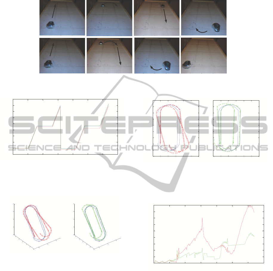
t=0s t=5s t=8s t=13s
t=16s t=21s t=29s t=32s
Figure 14: Snapshots of the experiment. In the straight line path the robot has a speed of 10.8cm/s. In the the circular path
the speed of the right wheel is 10.3cm/s and the left wheel is 17.5cm/s.
0 5 10 15 20 25 30 35
-50
0
50
100
150
200
250
300
350
400
Figure 15: Heading estimation. Solid blue line is the real
heading, solid red line is the heading estimation without ref-
erence system and solid green line is the heading estimation
with the reference system.
0
20
40
-20
0
20
40
60
80
-5
0
5
10
15
0
20
40
-20
0
20
40
60
80
-5
0
5
10
15
b)
a)
Figure 16: 3D position parameters, solid blue line is the
real path. a) Red circle is the position estimation without
reference system. b) Green circle is the position estimation
with reference system.
experiment.
Comparing the results in the figure, although both
methodologies have accumulative error over time, the
proposed reference system reduce significantly the
positioning error.
5 CONCLUSIONS
In this paper we have proposed a new 3D position-
ing algorithm for low cost robots. The architecture
presented can be applied in robots which have wheel
-10 0 10 20 30 40 50
-20
-10
0
10
20
30
40
50
60
70
-10 0 10 20 30 40 50
-20
-10
0
10
20
30
40
50
60
70
a)
b)
Figure 17: 2D position parameters (to show more clearly
the error, z has been set to zero), solid blue line is the real
path. a) Red circle is the position estimation without refer-
ence system. b) Green circle is the position estimation with
reference system.
0 5 10 15 20 25 30 35
0
2
4
6
8
10
12
14
16
18
Figure 18: Red solid line is the positioning error when the
reference system has not been used. The solid green line is
the positioning error when the reference system is used.
encoders and a three axis accelerometer. The prob-
lem formulation have been developed for two wheel
differential robots, however this algorithm is easy to
apply in other kind of robots in a simple way. The
methodology presented is based on a Finite State Ma-
chine. A threshold calculator allows to set the sys-
tem dynamically as a function of the noise in the
accelerometer. Also a new reference system is pro-
posed, this new system improves considerably the
estimation of the algorithm respect to the classical
odometry.
3DPositioningAlgorithmforLowCostMobileRobots
13

The proposed algorithm was checked in the low
cost robot mOway. In these experiments, in a simple
way, the algorithm has been set and precise estima-
tions of the 3D position were obtained. The thresh-
old calculator worked in a correct way to estimate the
states of the FSM and it sets the systems dynamically.
Finally with the new reference system the positioning
error has been considerably reduced.
As a future work, now we are considering to apply
this algorithm in robots which have also gyroscopesto
allow estimations on surface with elevation and bank
angles at the same time. On the other hand, newmeth-
ods for reference systems in low cost robots are being
explored.
REFERENCES
Abbas, T., Arif, M., and Ahmed, W. (2006). Measurement
and correction of systematic odometry errors caused
by kinematics imperfections in mobile robots. In
SICE-ICASE, 2006. International Joint Conference,
pages 2073–2078. IEEE.
Borenstein, J., Everett, H. R., Feng, L., and Wehe, D.
(1997). Mobile robot positioning-sensors and tech-
niques. Technical report, DTIC Document.
Borenstein, J. and Feng, L. (1995). Correction of system-
atic odometry errors in mobile robots. In Intelligent
Robots and Systems 95.’Human Robot Interaction and
Cooperative Robots’, Proceedings. 1995 IEEE/RSJ
International Conference on, volume 3, pages 569–
574. IEEE.
Everett, H. (1995). Sensors for mobile robots: theory and
application. AK Peters, Ltd.
Faisal, M., Hedjar, R., Alsulaiman, M., Al-Mutabe, K., and
Mathkour, H. (2014). Robot localization using ex-
tended kalman filter with infrared sensor. In Computer
Systems and Applications (AICCSA), 2014 IEEE/ACS
11th International Conference on, pages 356–360.
IEEE.
Jha, A. and Kumar, M. (2014). Two wheels differential
type odometry for mobile robots. In Reliability, Info-
com Technologies and Optimization (ICRITO)(Trends
and Future Directions), 2014 3rd International Con-
ference on, pages 1–5. IEEE.
Lee, Y.-C. and Park, S. (2014). Localization method for
mobile robots moving on stairs in multi-floor environ-
ments. In Systems, Man and Cybernetics (SMC), 2014
IEEE International Conference on, pages 4014–4020.
IEEE.
Liu, H. H. and Pang, G. K. (2001). Accelerometer for mo-
bile robot positioning. Industry Applications, IEEE
Transactions on, 37(3):812–819.
Luczak, S., Oleksiuk, W., and Bodnicki, M. (2006). Sens-
ing tilt with mems accelerometers. Sensors Journal,
IEEE, 6(6):1669–1675.
Roberson, R. E. and Schwertassek, R. (1988). Dynam-
ics of multibody systems, volume 18. Springer-Verlag
Berlin.
Seifert, K. and Camacho, O. (2007). Implementing posi-
tioning algorithms using accelerometers. Freescale
Semiconductor.
Siegwart, R., Nourbakhsh, I. R., and Scaramuzza, D.
(2011). Introduction to autonomous mobile robots.
MIT press.
Trimpe, S. and D’Andrea, R. (2010). Accelerometer-
based tilt estimation of a rigid body with only rota-
tional degrees of freedom. In Robotics and Automa-
tion (ICRA), 2010 IEEE International Conference on,
pages 2630–2636. IEEE.
ICINCO2015-12thInternationalConferenceonInformaticsinControl,AutomationandRobotics
14
