
Integrated Operations Planning for a Multicomponent Machine
Subjected to Stochastic Environment
Jean-Baptiste Ringard
1
, Bhushan S. Purohit
2
and Bhupesh Kumar Lad
2
1
Industrial and Logistics Systems, French Institute for Advanced Mechanics, Clermont-Ferrand, France
2
Discipline of Mechanical Engineering, Indian Institute of Technology Indore, Indore, India
Keywords: Integrated Planning, Supplier Planning, Scheduling, Preventive Maintenance, Simulation, Optimization.
Abstract: Operations management decisions related to production, maintenance, inventory and supplier selection has
attracted researchers since long. Traditionally each of these areas was planned and optimized individually.
Soon interdependencies between these elements of value chain were realized, which prompted researchers
towards integrated planning of these functions. Superiority of integrated approach over conventional
operations management approaches has already been demonstrated in past. Therefore, models integrating
shop floor functions like production planning, maintenance planning and inventory planning are abundant in
recent literature. However, there exist functions which significantly contribute towards operations planning,
but have still not been considered for integration. One such important area is procurement planning
(supplier order allocation).Current work aims to integrate procurement decisions with maintenance and
production plan so as to minimize Total Cost of Operations (TCO). It considers a stochastic environment
where production and maintenance processes are imperfect and where there is significant dubiety related to
demand and supply of material. Further, present model considers uncertainties in parameters like supplier
quality, machine yield etc., by using appropriate probability distributions for these parameters. Therefore a
simulation based Genetic Algorithm (GA) approach is used to solve this optimization problem. The final
results are illustrated in the form of an integrated operations plan. It explicitly communicates (i) Order
quantity for individual suppliers (ii) Job production sequence (iii) Production lot size (iv) Preventive
maintenance schedule for individual machine components. Current work aims to contribute towards
development of a paradigm where multiple disjoint functions are integrated at planning level itself.
1 INTRODUCTION
Fulfilling customer’s requirement is of prime
importance to all the organizations. These
requirements are fulfilled when all the functions of
the organization are aligned and perform efficiently.
Production, maintenance, quality and supply
management are few of such critical functions.
Supply management facilitates the availability of
raw material for production. Production is then
carried out through well maintained machines which
contribute towards good quality of products, which
are finally delivered to customers. In between,
inventory acts as cushion to accommodate
uncertainties and ensures availability of material.
Thus each of these functions together forms a strong
channel through which customer demand is realized.
Emphasizing on individual function, from a
diverse supplier base, supply management function
identifies suppliers which best fulfils the criteria like
capacity, capability and cost. Optimization of supply
management is linked with decisions like order
allocation, order quantities etc. On the production
planning front, job scheduling, manufacturing lot
size, allocation of job to different machine etc. are
amongst the key decisions to be optimized.
Similarly, which component / components to select
for preventive maintenance and when to perform
preventive maintenance are the decisions which
affect effectiveness of maintenance function. Similar
to such decisions is the decision related to inventory
management of raw materials and finished goods.
Extra inventory is considered to be waste as it calls
for capital expenditure which could otherwise be
used elsewhere. On the other hand fewer inventories
may lead to risk of material unavailability and may
result into non fulfilment of customer demand on
time.
Conventionally, planning of above mentioned
functions is performed individually. After individual
55
Ringard J., Purohit B. and Kumar Lad B..
Integrated Operations Planning for a Multicomponent Machine Subjected to Stochastic Environment.
DOI: 10.5220/0005496500550062
In Proceedings of the 5th International Conference on Simulation and Modeling Methodologies, Technologies and Applications (SIMULTECH-2015),
pages 55-62
ISBN: 978-989-758-120-5
Copyright
c
2015 SCITEPRESS (Science and Technology Publications, Lda.)

function’s plans are finalized, they are
communicated to other functions. However, during
execution of these plans, priorities of individual
functions do clash. Supply management may plan all
the material at once to reduce the ordering cost,
impacting the raw material inventory carrying cost.
Similarly, production may plan to manufacture the
maximum quantity so as to reduce cost related to
changeover, set-up etc. This increases the finished
good carrying cost. Also, it may deprive machine for
getting timely preventive maintenance leading to
catastrophic machine failure. Such failures calls for
prolonged corrective maintenance actions and also
affects quality of produced goods.
It is thus evident that performance of one
function severely affects performance of the others.
It therefore becomes imperative that the planning of
these functions must be carried out using an
integrated approach. Present paper aims to integrate
decisions related to supply management with that of
production, maintenance and inventory. In
particular, it aim to integrates supplier selection and
order quantity with shopfloor decisions like job
production sequence, manufacturing lot size and
preventive maintenance schedule.
2 LITERATURE REVIEW AND
PAPER CONTRIBUTION
Operations’ planning has gradually evolved from
optimization of individual parameters in a simplistic
environment to multi criteria optimization under
much complex environment. On scheduling, (Jones
et al., 1999) and (Chan et al., 2013), has
exhaustively reviewed the models developed for job
shop scheduling. Literature can also be found on
development of scheduling models for specific
objectives like minimizing job tardiness (Adamu and
Adewumi, 2014), or sequencing under uncertain
environment (Mula et al., 2006).
On the maintenance front the research expands
from maintenance optimization (Sharma et al., 2011)
to maintenance performance (Kumar et al., 2013).
Brief consolidation of the development in the field
of maintenance is mentioned in review by (Garg and
Deshmukh, 2006) for identifying the on-going trend
and future directions.
Concurrently, research has also progressed in the
field for supply management. Numerous decision
making approaches were proposed for optimizing
the decisions related to supplier selection as
mentioned in (Wilson, 1994). Review by (Aissaoui
et al., 2007) concentrates on mainly such models. It
proposes different classifications of the multiple
models which were published over the time.
Recent literature reflects that current focus of
researchers is towards the development of
“integrated” approaches (Hadidi et al., 2012).
There exist models which successfully integrate:
Production and Maintenance (Zhao et al., 2014)
Maintenance and Quality (Alfares et al., 2005)
Quality and Inventory (Peters et al., 1988)
Literature mentioned above demonstrates superiority
of integrated models compared to conventional
models. However, it can be noticed that all the
efforts for integration were confined mainly to
production, maintenance, inventory and quality. But,
there exists other equally critical functions beyond
those mentioned above, which also contributes
significantly towards the overall performance of
organization, but have been overlooked for
integration. Current work is an attempt to extend the
existing integrated models by incorporating one such
function namely Procurement Planning / Supply
Planning.
3 INDUSTRIAL PROBLEM
DISCRIPTION
The problem considers a multi component machine
as the central element of a small value chain with
customers at its one end and raw material suppliers
at the other end. Each customer can demand variety
of products in random quantity, to be delivered by
specific date. This demand needs to be processed on
a machine in a sequence which optimizes the total
cost of operations. To ensure the availability and
quality of output of machine, maintenance becomes
essential. Timely preventive maintenance is
performed in addition to corrective maintenance,
which is performed at the time of random machine
failure. Aligned with demand from each customer
and accounting for uncertainties, raw materials are
ordered from the set of previously screened
suppliers.
To elaborate further, consider a multi component
machine. Let the component be labelled as C
i
(0
,∈. The components are reliability wise
mutually independent and are in series. Time to
failure for each of these components follows two
parameter Weibull distributions, having shape
parameter and scale parameter as β
k
and η
k
respectively. These distribution parameters, along
with other factors, affect the stochastic failure of
SIMULTECH2015-5thInternationalConferenceonSimulationandModelingMethodologies,Technologiesand
Applications
56

components. Such failure can be reduced if timely
preventive maintenance (PM) action is performed as
each well planned PM activity positively influences
the life and performance of the machine.
Effectiveness of PM is measured as the factor by
which the life of the component can be restored and
is denoted by restoration factor (R). Though PM is
beneficial, it incurs time and resources which could
otherwise be used elsewhere. However in the
absence of PM, machine deteriorates speedily and
leads to frequent random failures. Such random
failures are addressed by corrective maintenance
(CM). Since causes of abrupt breakdowns are unsure
and CM activities are unplanned, they tend to
consume more time as compared to PM activities. It
is therefore necessary to carefully plan overall
maintenance schedule.
The manufacturing process carried out on the
machine is also imperfect in nature. An imperfect
process implies that the output will not always be
perfect and certain normal rejections are bound to
occur which affects the yield of the machine. The
machine is used to process the demand of multiple
products in different quantities from various
customers. This demand can be forecasted using
past records for each product and each customer.
The forecasted demand of individual product is
consolidated and further augmented by considering
the variability in the machine yield.
This augmented demand for products it
translated in to raw material requirements which is
to be fulfilled by group of previously identified
suppliers. The distribution of raw material order
quantity amongst the supplier is based on their
performance indicator like quality rating, cost,
discounts and capacity. Normal rejections are
expected from raw material supplied by supplier and
therefore quality rating refers to percentage of “OK”
parts received by suppliers. This rating is influenced
by operations at supplier’s end which are again
stochastic in nature and therefore considered as
normally distributed.
Machine is assumed to work for 16 hours per day
for 25 days in a month. In case the customer order
cannot be completed before due date, there is a
delayed delivery cost which is imposed by customer.
There is also a backorder cost which is imposed if
the delivered quantity is less than the ordered
quantity from supplier. Such backorders are lost
forever and are not added to requirement for next
month.
For a multi component machine, the problem lies
in preparing an optimized operations plan which
precisely quantifies conflicting decisions related to
production, maintenance and procurement while
accommodating uncertainties.
4 MATHEMATICAL MODAL
As stated above, using an integrated approach,
current work aims at minimizing the total cost of
operation. Total cost of operation (TCO) is
calculated as:
TCO = TMC+TCOPM+TCOCM+TBOC+
TDDC+TICC +TPC
Where,
TMC =Total Machining Cost
TCOPM = Total Cost of PM
TCOCM= Total Cost of CM
TBOC = Total Backorder Cost
TDDC = Total Delayed Delivery Cost
TICC =Total Inventory Carrying Cost
TPC = Total Procurement Cost
Individual models for above mentioned cost
components are mentioned here under.
If “s” be the number of suppliers, “m” be the
number of months in planning horizon, “p” be
number of products and “k” be the number of
components in the machine, then:
4.1 Machining Cost
If q
ij
is the manufactured quantity of product p
i
in j
th
month and
is machining time for i
th
product,
then Total manufacturing cost (TMC) is calculated
as:
q
(1)
4.2 Maintenance Cost
Total cost of preventive maintenance (TCOPM) is
calculated as:
TCOPM
(2)
where
is preventive maintenance factor for
k
th
component before p
th
production run in j
th
month
such that,
1
0
(3)
IntegratedOperationsPlanningforaMulticomponentMachineSubjectedtoStochasticEnvironment
57

is the time to perform preventive
maintenance on k
th
component. is the
maintenance labour cost per hour. Similarly, Total
Cost for Corrective Maintenance (TCOCM), is
calculated as:
TCOCM
(4)
where
is time to perform corrective
maintenance of k
th
component.
is number of
failures of k
th
component during p
th
production run in
j
th
month.
is calculated using formula published by
(Lad and Kulkarni, 2012)
Ƞ
Ƞ
(5)
where
is machining time for p
th
production run
in j
th
month. Ƞ
, and
are scale and shape
parameter of k
th
component respectively.
is the
initial age of k
th
component before p
th
production run
in j
th
month.
4.3 Backorder Cost
Total cost of backorder, (TBOC) is calculated as:
(6)
where,
is the backorder cost for i
th
product.
4.4 Delayed Delivery Cost
This is a penalty cost which is imposed by customer
in case the delivery of products is made after the
committed due date. It is calculated as:
(7)
Where,
0
,
,
(8)
where
and
are the actual delivery
date and committed delivery date respectively for
the i
product in j
th
month from c
th
customer.
is
the penalty cost per hour for the i
job and c
th
customer.
4.5 Inventory Carrying Cost
The goods which are left over after fulfilling the
monthly demand of customers are stored till next
delivery and thus cost extra for their storage.
Inventory carrying cost is the cost of stocking these
extra units.
(9)
where
is the inventory carrying cost for i
product and
is the extra units produced, if any.
4.6 Procurement Cost
It is the sum of ordering cost and material cost i.e.
Procurement Cost (PC) = Ordering Cost (OC) +
Material Cost (MC).
Each supplier has a different procedure for
processing the order and thus has different ordering
cost. Therefore total ordering cost is the sum of
ordering cost for each product from respective
supplier / suppliers. Total Ordering cost (TOC) is
calculated as:
(10)
where
supplier selection factor for p
th
product for s
th
supplier in j
th
month, such that is
1 if supplier is selected for delivering p
th
product and
“0” otherwise
Total Material Cost is the product of unit price of
product, discount factor, quantity ordered and
supplier selection factor. It can be mathematically
written as:
(11)
Where
is the quantity ordered of i
th
product by s
th
supplier in j
th
month and
and
is the unit
price and discount factor for of i
th
product by s
th
supplier.
SIMULTECH2015-5thInternationalConferenceonSimulationandModelingMethodologies,Technologiesand
Applications
58

Table 1: Machine Component Characteristics.
k
th
Component
Initial Age
(hours) Ia
k
Scale
factor
η
k
Shape
factor
β
k
Restoration
factor for PM
R
k
PM Fixed
Time
CM
Fixed
Time
CM Variable Time
(hours)
Mean
μ
k
Standard
Deviation
σ
k
1
st
Component 3000 1200 2 0.5 3 1 8 2
2
nd
Component 3000 900 2.5 0.5 3 1 8 2
3
rd
Component 3000 1100 3 0.5 3 1 8 2
4
th
Component 3000 600 1.5 0.5 3 1 8 2
5
th
Component 3000 1500 1.8 0.5 3 1 8 2
5 NUMERICAL EXAMPLE AND
RESULTS
To illustrate the above mentioned model, consider a
multi component machine with five components
with characteristics as mentioned in table 1.This
machine manufactures four different products
namely P1, P2, P3 and P4 .Characteristics of these
products are as shown in table 2 and 3.
Table 2: Product Characteristics.
Product
P1 P2 P3 P4
Manufacturing time (Hours) 0.2 0.25 0.22 0.25
Labor Cost per hour 60 60 60 60
Inventory carrying cost Per Unit 0.25 0.25 0.25 0.25
Table 3: Due Dates and Penalty Costs.
P1 P2 P3 P4
Due date
(Days)
Customer 1 15 15
Customer 2 18 18
Customer 3 17 17 17
Customer 4 16 16 16
Penalty cost
/per hours
delay
Customer 1 7 7
Customer 2 8 8
Customer 3 5 5 5
Customer 4 9 6 6
Back Order
Cost Per Unit
Customer 1 68 68
Customer 2 70 70
Customer 3 72 72 72
Customer 4 69 69 69
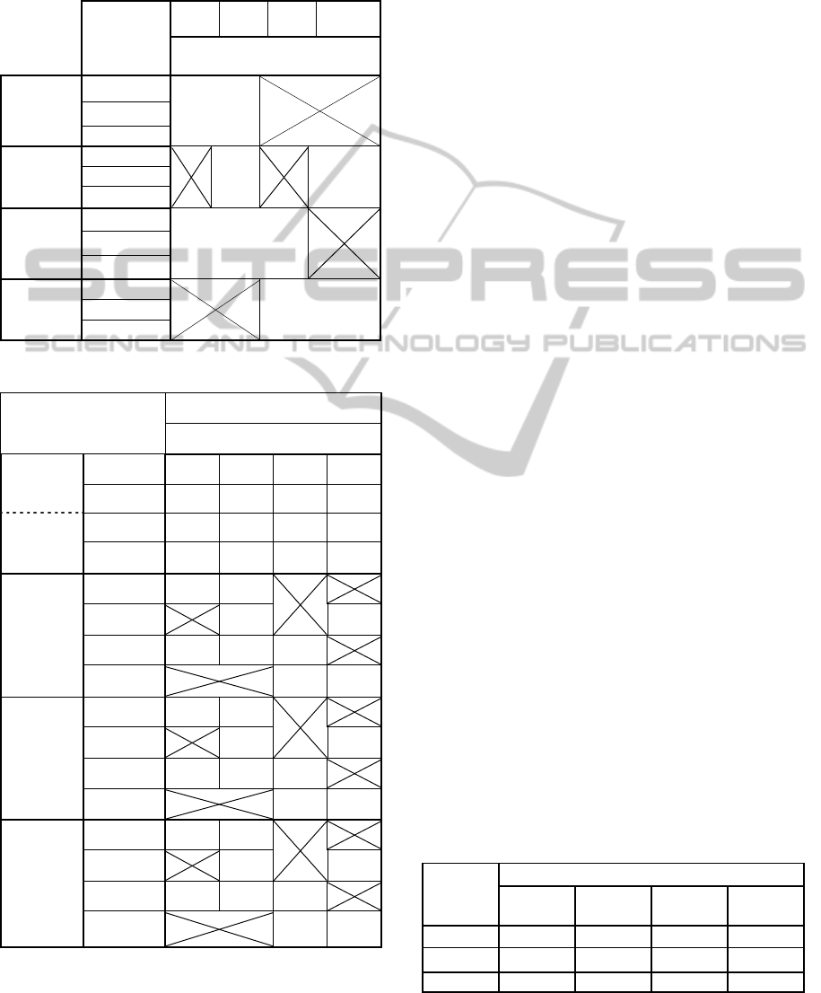
These products can be demanded from multiple
customers. The monthly demand of each product for
the products is forecasted. However, actual demand
is uniformly distributed and uncertain. The demand
pattern for a month is as mentioned in table 4.
Material planner orders raw material by
considering forecasted demand, average supplier
quality rating and average percentage rejections at
machine. The raw material order quantity is thus
calculated as:
OQ
FD
/
SQR
MQR
(12)
where,OQ
= Order quantity for raw material of i
th
product in j
th
month, FD
is forecasted demand of i
th
product in j
th
month, SQR
is average supplier
quality rating for i
th
product and MQR
is machine
quality rating for i
th
product.
Table 4: Monthly Demand.
C= Customer
Product
P1 P2 P3 P4
Demand
Forecast
(units)
C1 90 90
C2 85 95
C3 85 95 85
C4 95 95 100
Aggregate of
Demand Forecast
175 280 265 195
Uniformly
Distributed
Actual
Demand
(units)
C1 81-99 81-99
C2 76-94 85-105
C3 76-94 85-105 76-94
C4 85-105 85-105 90-110
Aggregate of Actual
demand
157-193 251-309
237-
293
175-
215
The organization follows multi sourcing policy
which means that order quantity of raw material for
these products can be split amongst the set of
IntegratedOperationsPlanningforaMulticomponentMachineSubjectedtoStochasticEnvironment
59
previously identified suppliers. This split or
distribution of order is influenced by supplier
performance indicator like cost, quality rating etc.
Table 5: Discount Window.
Order
Quantity
RM1 RM2 RM3 RM4
Percentage Discount for
per unit cost
Supplier 1
0 to 176 0 0
177 to 235 9 10
above 235 15 16
Supplier 2
0 to 179
0
0
180 to 239 10 9
above 240 16 17
Supplier 3
0 to 158 0 0 0
159 to 211 7 7 7
above 212 12 12 12
Supplier 4
0 to 170
0 0
171 to 227 6 6
above 227 11 12
Table 6: Supplier Details.
Raw Material
RM 1 RM 2 RM 3 RM 4
1 = Can
Supply
Supplier 1 1 1 0 0
Supplier 2 0 1 0 1
0= Cannot
supply
Supplier 3 1 1 1 0
Supplier 4 0 0 1 1
Cost/ Unit
Ordered
Supplier 1 1.5 1.6
Supplier 2
1.7 1.7
Supplier 3 1.75 1.75 1.75
Supplier 4
1.6 1.6
Maximum
Order
Quantity
Supplier 1 300 295
Supplier 2
300 300
Supplier 3 265 265 265
Supplier 4
285 285
Average
Quality
Rating
(%)
Supplier 1 0.96 0.96
Supplier 2
0.97 0.95
Supplier 3 0.94 0.94 0.93
Supplier 4
0.97 0.99
Also, to attract large orders, suppliers provides
discounted price for larger ordered quantities. Such
supplier characteristics are as mentioned in table 5
and table 6.
6 SOLUTION METHOD
In general, conventional “M Job-1 Machine”
production scheduling problem have M! feasible
solution. Likewise, maintenance decision for a
particular component is binary in nature – PM or No
PM. Thus, for a machine with “k” components, PM
activity leads to 2
k
possible decisions. This
maintenance decision is repeated after each of the
“M” production run for “m” months, which leads to
total no. of solutions as [(M!)(2
k
)
M
]
m
. For the
example mentioned above, M=4, k=5 and m=3,
which leads to total number of feasible solution
equal to 1.5
22
approximately. This number excludes
the decision variable related to, production lot size,
supplier selection and order quantity which
manifolds the number of possible solutions. Such
combinatorial situations, makes it complex to use
any exact algorithm.
In addition, present models also incorporate
uncertainties in machine yield, actual demand,
supplier quality rating and other parameters. Such
considerations are accommodated to closely
replicate real world complexities. This is achieved
using probability distributions for value of specific
parameters mentioned above. Therefore a simulation
based Genetic algorithm approach is used to solve
this optimization problem. “@ RISK” optimizer”
software is used for the same in this research.
7 RESULTS
The model was simulated for over one lakh trials,
each having 50 iterations, for generating optimized
results. A part of optimization log is as mentioned in
table 7. The table shows that minimum cost is
obtained in trial no. 88780. No further reduction in
cost was observed after this trial and thus log is
truncated at this trial number.
Table 7: Log of Progress Steps.
Trial
Goal Cell Statistics
Min. Max. Std. Dev.
Result
(Mean)
23259 123874 140410 6522 134221
28414 123874 139423 6140 133862
88780 123960 138952 5894
133455
SIMULTECH2015-5thInternationalConferenceonSimulationandModelingMethodologies,Technologiesand
Applications
60
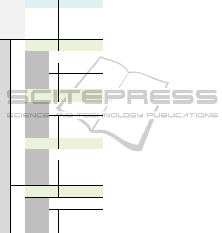
Table 8: Integrated Operations Plan (IOP).
Monthly
Procurement
Decision
Supplier S1 S2 S3 S4
Order
Quantity
P1 100 100
P2 100 100 0
P3 121 169
P4 202 0
PRODUCTION RUN
RUN 1
Product to be
Manufactured
P2 Lot Size 193
Preventive
Maintenance
Decision
(1=Execute
PM,
0=No PM)
Component
C1 C2 C3 C4 C5
0 1 0 0 0
RUN 2
Product to be
Manufactured
P1 Lot Size 182
Preventive
Maintenance
Decision
(1=Execute
PM,
0=No PM)
Component
C1 C2 C3 C4 C5
0 0 0 0 0
RUN 3
Product to be
Manufactured
P3 Lot Size 275
Preventive
Maintenance
Decision
(1=Execute
PM,
0=No PM)
Component
C1 C2 C3 C4 C5
0 0 1 0 0
RUN 4
Product to be
Manufactured
P4 Lot Size 191
Preventive
Maintenance
Decision
(1=Execute
PM,
0=No PM)
Component
C1 C2 C3 C4 C5
0 1 0 0 0
The decisions corresponding to this optimal
solution are represented in the form of a unified
operations plan as summarized in table 8.
From the table it can be noted that, in order to
have minimum total cost of operation, for the month
of January, the schedule proposes total order
quantity as 200, 302, 221 and 169 from S1, S2, S3
and S4 respectively. Simultaneously, it also
proposes the production sequence as P2, P1, P3, and
P4 with respective manufacturing quantities as 193,
182, 275 and 191 as highlighted in the table. It also
integrates optimized preventive maintenance plan as
mentioned under column “Individual component
maintenance decision” by showing “1” for
components which needs to go for preventive
maintenance after each production run.
To summarize, this integrated operations plan
precisely communicates decisions related to:
1. Production
Job sequencing
Manufacturing lot size
2. Maintenance
PM schedule for individual components
3. Procurement
Supplier Selection
Order Quantity
8 CONCLUSIONS
Functions like production, maintenance, inventory
etc. have already been combinatorialy considered for
integration. However, with addition of each
function, complexity of formulating an integrated
model manifolds which apprehends the integration
of more functions for operations planning. Current
work successfully fills this gap by exhaustive
integration of multiple functions viz. production,
maintenance, inventory and procurement. In
addition, it incorporates stochastic nature of the
processes like imperfect machining and maintenance
process which brings it closer to real manufacturing
environment. Consequently, current work can be
looked upon as a step towards development over
existing models which lacks integration to a detailed
level where parameters and constraints related to
processes, equipment etc. are also taken into account
for integration.
REFERENCES
Jones, A., Rabelo, L. C., & Sharawi, A. T., 1999. Survey
of job shop scheduling techniques. Wiley
Encyclopedia of Electrical and Electronics
Engineering.
Chan, H. K., Chung, S. H., & Lim, M. K., 2013. Recent
research trend of economic-lot scheduling problems.
Journal of Manufacturing Technology Management,
24(3), 465-482.
Adamu, M. O., & Adewumi, A. O., 2014. A survey of
single machine scheduling to minimize weighted
number of tardy jobs. Journal of Industrial and
Management Optimization, 10(1), 219-241.
IntegratedOperationsPlanningforaMulticomponentMachineSubjectedtoStochasticEnvironment
61

Mula, J., Poler, R., Garcia-Sabater, J. P., & Lario, F. C.,
2006. Models for production planning under
uncertainty: A review. International journal of
production economics, 103(1), 271-285.
Sharma, A., Yadava, G. S., & Deshmukh, S. G., 2011. A
literature review and future perspectives on
maintenance optimization. Journal of Quality in
Maintenance Engineering, 17(1), 5-25.
Kumar, U., Galar, D., Parida, A., Stenström, C., & Berges,
L., 2013. Maintenance performance metrics: a state-
of-the-art review. Journal of Quality in Maintenance
Engineering, 19(3), 233-277.
Garg, A., & Deshmukh, S. G., 2006. Maintenance
management: literature review and directions. Journal
of Quality in Maintenance Engineering, 12(3), 205-
238.
Wilson, E. J., 1994. The relative importance of supplier
selection criteria: a review and update. International
Journal of Purchasing and Materials Management,
30(2), 34-41.
Aissaoui, N., Haouari, M., & Hassini, E., 2007. Supplier
selection and order lot sizing modeling: A review.
Computers & operations research, 34(12), 3516-3540.
Hadidi, L. A., Al-Turki, U. M., & Rahim, A., 2012.
Integrated models in production planning and
scheduling, maintenance and quality: a review.
International Journal of Industrial and Systems
Engineering, 10(1), 21-50.
Zhao, S., Wang, L., & Zheng, Y., 2014. Integrating
production planning and maintenance: an iterative
method. Industrial Management & Data Systems,
114(2), 162-182.
Alfares, H. K., Khursheed, S. N., & Noman, S. M., 2005.
Integrating quality and maintenance decisions in a
production-inventory model for deteriorating items.
International Journal of Production Research, 43(5),
899-911.
Peters, M., Schneider, H. & Tang, K., 1988. ‘Joint
determination of optimal inventory and quality control
policy’, Management Science, Vol. 34, No. 8, pp.
991–1004.
Lad, Bhupesh Kumar, & Makarand S. Kulkarni, 2012.
Optimal Maintenance Schedule Decisions for Machine
Tools Considering the User's Cost Structure,
International Journal of Production Research 50, no.
20: 5859-5871.
SIMULTECH2015-5thInternationalConferenceonSimulationandModelingMethodologies,Technologiesand
Applications
62
