
A Model Predictive Sliding Mode Control with Integral Action for
Slip Suppression of Electric Vehicles
Tohru Kawabe
Faculty of Engineering, Information and Systems, University of Tsukuba, Tsukuba 305-8573, Japan
Keywords:
Electric Vehicle, Slip Ratio, Robustness, Sliding Mode Control, Model Predictive Control.
Abstract:
This paper proposes a new SMC (Sliding Mode Control) method with MPC (Model Predictive Control) al-
gorithm for the slip suppression of EVs (Electric Vehicles). This method introducing the integral term with
standard SMC gain, where the integral gain is optimized for each control period by solving an optimization
problem based on the MPC algorithm to improve the acceleration performance and the energy consumption
of EVs. Numerical simulation results are also included to demonstrate the effectiveness of the method.
1 INTRODUCTION
Over the past decades, the automobile population has
been increasing rapidly in the developing countries,
such as BRICs (Brazil, Russia, India and China) (Dar-
gay et al., 2007). With the wide spread of automobiles
all over the world, especially internal-combustion en-
gine vehicles (ICEVs), the environment and energy
problems: air pollution, global warming, oil resource
exhaustion and so on, are going severely (Mamalis
et al., 2013). As a countermeasure to these prob-
lems, the development of next-generation vehicles
have been focused. EVs run on electricity only and
they are zero emission and eco-friendly. So EVs have
attracted great interests as a powerful solution against
the problems mentioned above (Brown et al., 2010;
Hirota et al., 2011; Tseng et al., 2013).
EVs are propelled by electric motors, using elec-
trical energy stored in batteries or another energy stor-
age devices. Electric motors have several advantages
over ICEs (Internal-Combustion Engines):
• The input/output response is faster than for gaso-
line/diesel engines.
• The torque generated in the wheels can be de-
tected relatively accurately
• Vehicles can be made smaller by using multiple
motors placed closer to the wheels.
The travel distance per charge for EV has been in-
creased through battery improvements and using re-
generation brakes, and attention has been focused on
improving motor performance. The above-mentioned
facts are viewed as relatively easy ways to improve
maneuverability and stability of EVs.
It’s, therefore, important to research and develop-
ment to achieve high-performance EV traction con-
trol. Several methods have been proposed for the
traction control (Fujii and Fujimoto, 2007) by us-
ing slip ratio of EVs, such as the method based
on MFC (Model Following Control) in (Hori, 2000)
We have been proposed MP-PID (Model Predictive
Proportional-Integral-Derivative) method in (Kawabe
et al., 2011) and MP-2DOF-PID method in (Kawabe,
2014).
These methods show good performances under
the nominal conditions where the situations, for ex-
ample, mass of vehicle, road condition, and so on,
are not changed. To meet the high performance even
variation happened in such conditions, it is signifi-
cant to construct the robust control systems against
the changing of situation. About this point, SMC per-
forms good robustness against the uncertainties and
nonlinearities of the systems.
However, for slip suppression with the conven-
tional SMC (Slotine and Li, 1991; Eker and Aki-
nal, 2008) , the control performance will get degrada-
tion due to the chattering which always occurs when
switching the control inputs due to the structure of
SMC. To overcome such disadvantages, the SMC
method introducing the integral action with gain to
design the sliding surface (SMC-I) has been proposed
in (Li and Kawabe, 2013), where the integral gain
is derived by trial and error. In order to get better
control performance and save more energy for slip
suppression of EVs with changing the mass of vehi-
151
Kawabe T..
A Model Predictive Sliding Mode Control with Integral Action for Slip Suppression of Electric Vehicles.
DOI: 10.5220/0005500401510158
In Proceedings of the 12th International Conference on Informatics in Control, Automation and Robotics (ICINCO-2015), pages 151-158
ISBN: 978-989-758-123-6
Copyright
c
2015 SCITEPRESS (Science and Technology Publications, Lda.)
cle and road condition, the optimal gain derived on-
line is expected. Therefore, we have developed the
Model Predictive Sliding Mode Control with Integral
action (MP-SMC-I) (Li and Kawabe, 2014), which
determines the integral gain adaptively at each step by
MPC algorithm (Maciejowski, 2005). However, there
are some room to improve the robust performance of
this method. This paper, therefore, proposes the im-
proved MP-SMC-I method. The simulation results
are shown to verify the effectiveness of the proposed
method.
2 ELECTRIC VEHICLE
DYNAMICS
As a first step toward practical application, this paper
restricts the vehicle motion to the longitudinal direc-
tion and uses direct motors for each wheel to simplify
the one-wheel model to which the drive force is ap-
plied. In addition, braking was not considered this
time with the subject of the study being limited to
only when driving.
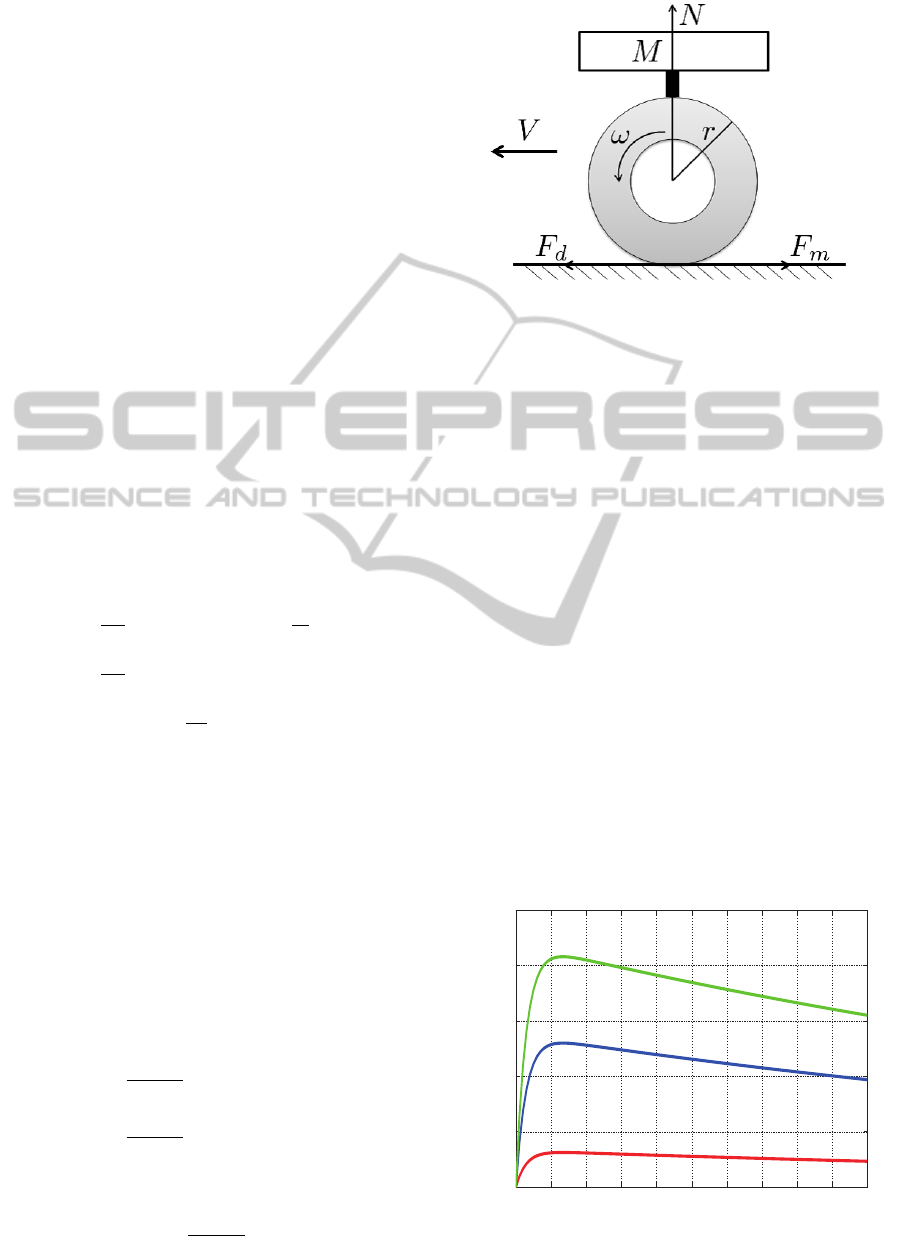
From fig. 1, the vehicle dynamical equations are
expressed as eqs. (1) to (4).
M
dV
dt
= F
d
(λ) − F
a
−
T
r
r
(1)
J
dω
dt
= T
m
− rF
d
(λ) − T
r
(2)
F
m
=
T
m
r
(3)
F
d
= µ(c,λ)N (4)
Where M is the vehicle weight, V is the vehicle body
velocity, F
d
is the driving force, J is the wheel inertial
moment, F
a
is the resisting force from air resistance
and other factors on the vehicle body, T
r
is the fric-
tional force against the tire rotation, ω is the wheel
angular velocity, T
m
is the motor torque, F
m
is the
motor torque force conversion value, r is the wheel
radius, and λ is the slip ratio. N is the normal tire
force defined as N = Mg where g is the acceleration
of gravity. The slip ratio is defined by eq. (5) from the
wheel velocity (V
ω
) and vehicle body velocity (V ).
λ =
V
ω
−V
V
ω
(accelerating)
V −V
ω
V
(braking)
(5)
λ during accelerating can be shown by eq. (6) from
fig. 1.
λ =
rω −V
rω
(6)
Figure 1: One-wheel car model.
The frictional forces that are generated between
the road surface and the tires are the force generated
in the longitudinal direction of the tires and the lateral
force acting perpendicularly to the vehicle direction
of travel, and both of these are expressed as a func-
tion of λ. The frictional force generated in the tire
longitudinal direction is expressed as µ, and the rela-
tionship between µ and λ is shown by eq. (7) below,
which is a formula called the Magic-Formula(Pacejka
and Bakker, 1991) and which was approximated from
the data obtained from testing.
µ(λ) = −c
road
× 1.1 × (e
−35λ
− e
−0.35λ
) (7)
Where c
road
is the coefficient used to determine the
road condition and was found from testing to be ap-
proximately c
road
= 0.8 for general asphalt roads, ap-
proximately c
road
= 0.5 for general wet asphalt, and
approximately c
road
= 0.12 for icy roads. For the var-
ious road conditions (0 < c < 1), the µ − λ surface is
shown in fig. 2.
It shows how the friction coefficient µ increases
with slip ratio λ (0.1 < λ < 0.2) where it attains the
maximum value of the friction coefficient. As defined
in eq. (4), the driving force also reaches the maximum
0 0.1 0.2 0.3 0.4 0.5 0.6 0.7 0.8 0.9 1
0
0.2
0.4
0.6
0.8
1
Slip Ratio λ
Friction coecient µ
Icy road
Wet asphalt road
Dry asphalt road
Figure 2: µ − λ curve for road conditions.
ICINCO2015-12thInternationalConferenceonInformaticsinControl,AutomationandRobotics
152

value corresponding to the friction coefficient. How-
ever, the friction coefficient decreases to the minimum
value where the wheel is completely skidding. There-
fore, to attain the maximum value of driving force for
slip suppression, it should be controlled the optimal
value of slip ratio. the optimal value of λ is derived as
follows. Choose the function µ
c
(λ) defined as
µ
c
(λ) = −1.1 × (e
−35λ
− e
−0.35λ
). (8)
By using eqs. (7) and (8), it can be rewritten as
µ(c,λ) = c
road
· µ
c
(λ). (9)
Evaluating the values of λ which maximize µ(c,λ)
for different c(c > 0), means to seek the value of λ
where the maximum value of the function µ
c
(λ) can
be obtained. Then let
d
dλ
µ
c
(λ) = 0 (10)
and solving equation (10) gives
λ =
log100
35 − 0.35
≈ 0.13. (11)
Thus, for the different road conditions, when λ ≈ 0.13
is satisfied, the maximum driving force can be gained.
Namely, from eq. (7) and fig. 2, we find that regard-
less of the road condition (value of c), the λ − µ sur-
face attains the largest value of µ when λ is the opti-
mal value 0 .13.
3 MP-SMC WITH INTEGRAL
ACTION DESIGN FOR SLIP
SUPPRESSION
3.1 SMC with Integral Action (SMC-I)
Method
In this section, the previous proposed control strategy
based on SMC with integral action (SMC-I) (Li and
Kawabe, 2013) is explained. Without loss of gener-
ality, one wheel car model in fig. 1 is used for the
design of the control law. The nonlinear system dy-
namics can be presented by a differential equation as
˙
λ = f + bT
m
(12)
where λ ∈ R is the state of the system representing the
slip ratio of the driving wheel which is defined as eq.
(5) for the case of acceleration, T
m
is the control in-
put. f describes the nonlinearity of system and b is
the input gain, and they are all time-varying. Differ-
entiating eq. (5) with respect to time gives
˙
λ =
−
˙
V + (1 − λ)
˙
V
w
V
w
(13)
and substituting eqs. (1), (2) and (4) into eq. (13), the
following equations can be attained,
f = −
g
V
w
1 + (1 − λ)
r
2
M
J
w
µ(c,λ), (14)
b =
(1 − λ)r
J
w
V
w
. (15)
The sliding mode controller is described to main-
tain the value of slip ratio λ at the desired value λ
∗
.
Referring to (Li and Kawabe, 2013), in order to
reduce the undesired chattering effect for which it is
possible to excite high frequency modes, and guaran-
tee zero steady-state error, an integral action with gain
has been introduced to the design of sliding surface.
By adding an integral item to the difference between
the actual and desired values of the slip ratio, the slid-
ing surface function s is given by
s = λ
e
+ K
in
∫
t
0
λ
e
(τ)dτ, (16)
where λ
e
is defined as λ
e
= λ− λ
∗
and K
in
is the inte-
gral gain, K
in
> 0.
The sliding mode occurs when the state reaches
the sliding surface defined by s = 0. The dynamics of
sliding mode is governed by
˙s = 0. (17)
By using eqs. (12) to (17), the sliding mode con-
trol law is derived by adding a switching control input
T
msw
to the nominal equivalent control input T
meq n
as
in (Li and Kawabe, 2013)
T
m
= T
meq n
+ T
msw
, (18)
T
meq n
=
1
b
[− f
n
− K
in
λ
e
], (19)
T
msw
=
1
b
−Ksat(
s
Φ
)
, (20)
sat
s
Φ
=
−1 s < −Φ
s
Φ
−Φ ≤ s ≤ Φ,
1 s > Φ
(21)
where “
n
” is used to indicate the estimated model
parameters. f
n
is the estimation of f calculated by us-
ing the nominal values of vehicle mass M
n
and road
surface condition coefficient c
n
. Φ > 0 is a design pa-
rameter which defines a small boundary layer around
the sliding surface. The sliding gain K > 0 is selected
as
K = F + η (22)
by defining Lyapunov candidate function in (Li and
Kawabe, 2013), where F = | f − f
n
| and η is a design
parameter.
By using eqs. (18), (19), (20) and (22), the control
law of SMC-I can be represented as
T
m
=
1
b
− f
n
− K
in
λ
e
− (F + η)sat
s
Φ
. (23)
AModelPredictiveSlidingModeControlwithIntegralActionforSlipSuppressionofElectricVehicles
153

3.2 Improved Model Predictive SMC
with Integrl Action (MP-SMC-I)
Method
In this section, we show the improved MP-SMC-I
method. Although the MP-SMC-I method has been
developed by us (Li and Kawabe, 2014), it has disad-
vantage to take time to calculate the predicted control
input (
ˆ
T
m
). Then we improved this point to propose
new calculation method.
Generally, MPC algorithm is used to predict the
future state behavior base on the discrete-time state
space model (Maciejowski, 2005) . The continuous
time state space model for the slip ratio control repre-
sented by eq. (12) can not be dealt with in the same
way. It is transformed to the discrete time state space
model at sampling time t = kT , T is the sampling pe-
riod. The torque input is defined by
T
m
(t) = T
m
(kT ), kT ≤ t < (k + 1)T. (24)
For convenience, we will omit T in the following
equations.
The controlled object of vehicle dynamics can be
described as follows.
λ(k + 1) = f
d
k, λ(k)
+ b
d
k, λ(k)
T
m
(k) (25)
where λ(k) is the state variable representing the slip
ratio at time k. f
d
k, λ(k)
describes the nonlinearity
of the discrete time system, b
d
k, λ(k)
is the input
gain, and they are given by
f
d
k, λ(k)
= −
g
V
w
(k)
1 +
1 − λ(k)
r
2
M
J
w
×µ
c,λ(k)
(26)
b
d
k, λ(k)
=
1 − λ(k)
r
J
w
V
w
(k)
. (27)
The control input T
m
(t) given by eq. (23) can be
rewritten as
T
m
(k) =
1
b
d
k, λ(k)
f
dn
k, λ(k)
− K
in
(k)
λ(k) − λ
∗
−
F
d
k, λ(k)
+ η
sat
s
k, λ(k),K
in
(k)
Φ
where λ
∗
is the reference slip ratio, η is the design pa-
rameter, and both of them are constants. f
dn
k, λ(k)
is the estimation of f
d
k, λ(k)
and is defined as
f
dn
k, λ(k)
=
−gµ
c
n
,λ(k)
V
w
(k)
1 +
1 − λ(k)
r
2
M
n
J
w
.
(28)
Now, we set current time to k. For a prediction
horizon H
p
, the predicted slip ratios
ˆ
λ(k + i) for i =
1,··· ,H
p
depend on the known values of current slip
ratios, current torque input and future torque inputs.
By using eq. (25), the predicted slip ratios can be
represented as
ˆ
λ(k + H
p
) = f
d
k + H
p
− 1,
ˆ
λ(k + H
p
− 1)
+ b
d
k + H
p
− 1,
ˆ
λ(k + H
p
− 1)
×
ˆ
T
m
(k + H
p
− 1) (29)
where
ˆ
T
m
(k + i), i = 0, · · · , H
p
− 1 are predicted con-
trol inputs.
ˆ
T
m
(k + i) is given by
ˆ
T
m
(k + i) =
f
dn
k + i,
ˆ
λ(k + i)
− K
in
ˆ
λ(k + i) − λ
∗
b
d
k + i,
ˆ
λ(k + i)
−
F
d
k + i,
ˆ
λ(k + i)
+ η
sat
s
k+i,
ˆ
λ(k+i),K
in
Φ
b
d
k + i,
ˆ
λ(k + i)
.
Where
F
d
k, λ(k)
=
g
V
w
k, λ(k)
µ
c
max
,λ(k)
− µ
c
n
,λ(k)
+
g
1 − λ(k)
r
2
J
w
V
w
k, λ(k)
M
max
µ
c
max
,λ(k)
− M
n
µ
c
n
,λ(k)
and where M
n
is the estimated value of vehicle mass
M and c
n
is estimated for the viscous friction coeffi-
cient c. This calculation method of
ˆ
T
m
is improved
method of previous our method (Li and Kawabe,
2014).
Here, we define the estimated values of these pa-
rameters respectively as the arithmetic mean of the
value of the bounds.
c
n
=
c
min
+ c
max
2
(30)
M
n
=
M
min
+ M
max
2
. (31)
Actually, the mass of the car often changes with the
number of passengers and the weight of luggage. Be-
sides, the car has to always travel on various road sur-
faces. Then the ranges of variation in parameter c and
parameter M are assumed to be defined as
c
min
≤ c ≤ c
max
(32)
M
min
≤ M ≤ M
max
. (33)
Here, the objective function J for deciding the
value of K
in
can be written as
ICINCO2015-12thInternationalConferenceonInformaticsinControl,AutomationandRobotics
154

J =
H
p
−1
∑
i=0
q|
ˆ
λ(k + i + 1) − λ
∗
| + r|
ˆ
T
m
(k + i)|
(34)
where q, r are the positive weights. By using eqs. (29)
and (30), both
ˆ
λ and
ˆ
T
m
can be expressed by K
in
, thus
J can be represented by a function of K
in
. Our aim
is to find the parameter K
in
that minimizes this objec-
tive function J(K
in
). In a nutshell, the optimization
problem is given by
min
K
in
J(K
in
)
s. t. [ Some constraint conditions
with input or output (if exist)] (35)
At time k, the optimal K
in
(k) can be found by solving
eq. (35) with some optimization method (here, a grid
search method is made to the discretized K
in
) by MPC
Algorithm. Once the optimal K
in
(k) is determined, it
is used as the continuous K
in
(t) for kT ≤ t < (k +
1)T , then the continuous control input T
m
(t) can be
calculated by eq. (23). At the next sampling time k +
1, the optimal K
in
(k + 1) is calculated as the previous
step. At each sampling period, the same operation
is repeated. Therefore, using the MP-SMC-I method
could determine the optimal parameter K
in
by solving
the optimization problem.
4 NUMERICAL EXAMPLES
4.1 Simulation Settings
This section shows the numerical simulation results to
demonstrate the effectiveness of the proposed method
as shown in previous section. The performance of the
proposed MP-SMC-I method is compared with that
of no-control, SMC and SMC-I methods. In the sim-
ulation examples, the vehicle starts from rest and ac-
celerates on icy road, wet asphalt road and dry as-
phalt road respectively with the parameters of dynam-
ics shown in table 1. The maximum simulation time is
set to 20[s] and the maximum velocity of the vehicle
is 180[km/h].
Table 1: Parameters used in the simulations.
J
w
:Inertia of wheel 21.1[kg/m
2
]
r:Radius of wheel 0.26[m]
λ
∗
:Desired slip ratio 0.13
g:Acceleration of gravity 9.81[m/s
2
]
The SMC controller parameters Φ,η as well as the
integral gain K
in
are listed in table 2 which are deter-
mined by trial and error.
Table 2: Controller settings
SMC Φ = 1,η = 5
SMC-I Φ = 1,η = 5
K
in
= 10
MP-SMC-I Φ = 1,η = 5
0 ≤ K
in
≤ 200, ∆K
in
= 1
q = 1.0 × 10
8
r = 1.0
In order to evaluate the energy consumption by
the electric motor, we estimate the energy consumed
for driving the wheel based on the following assump-
tions. Firstly, the electric power is all used to drive the
wheel. Secondly, the power consumed by the vehicle
is in proportional with the rotational energy due to the
rotation of driven wheel. The rotational energy E
rot
is
defined by the rotational inertia of wheel J
w
and the
angular velocity w is given by
E
rot
=
1
2
J
w
w
2
. (36)
In the simulations, the total distance traveled is calcu-
lated by integrating the vehicle velocity from 0 to the
simulation time t
int
and is defined as
D
dis
=
∫
t
int
0
V dt. (37)
To learn how much the energy consumed with respect
to the distance, the cost of the energy per distance (en-
ergy consumption rate) are also calculated.
4.2 Simulation Results
In order to verify the robustness of proposed MP-
SMC-I with variation both in the mass of vehicle and
road condition, the range of the uncertainties in the
mass of vehicle M is [1000,1400][kg] and the range of
road condition coefficient c is [0.1,0.9]. The nominal
values used in the controller design taking the arith-
metic mean of the edge values are M
n
= 1200[kg],
c
n
= 0.5.
Furthermore, three road surfaces switch in the
simulation by time as: an icy road (c = 0.12) dur-
ing [0,0.45)[s], another icy road (c = 0.20) dur-
ing [0.45, 8)[s], a wet asphalt road(c = 0.50) dur-
ing [8,9)[s] and a dry asphalt road(c = 0.80)) during
[9,10][s].
As shown in fig. 3, the slip ratio can be suppressed
to reference value 0.13 represented by black dot
line accurately and rapidly regardless of the masses
changing by 100[kg] from 1000[kg] to 1400[kg].
This implies that MP-SMC-I acts robustly to the vari-
ation in vehicle mass. It also makes a good transient
performance at the switching spots on the road condi-
tion.
AModelPredictiveSlidingModeControlwithIntegralActionforSlipSuppressionofElectricVehicles
155
0 1 2 3 4 5 6 7 8 9 10
0
0.2
0.4
0.6
0.8
1
Time [s]
Slip ratio
b
b
M=1000[kg]
M=1100[kg]
M=1200[kg]
M=1300[kg]
M=1400[kg]
Reference value
Figure 3: Time response of slip ratio with MP-SMC-I for
different vehicle masses.
Next, we compared MP-SMC-I with the conven-
tional SMC, SMC-I and no control. For saving of
space, only results with the case of vehicle mass
M assigned to 1000[kg] and 1400[kg] are limited to
shown below. From figs. 4 and 5 show the responses
of slip ratio and motor torque under three different
road conditions. The slip ratio by MP-SMC-I can
be suppressed to the reference value more accurately
and rapidly than SMC-I. When the road condition
changes, the slip ratio by MP-SMC-I also keep an
suitable transient performance, reducing the steady
0 1 2 3 4 5 6 7 8 9 10
0
0.2
0.4
0.6
0.8
1
Time [s]
Slip ratio
No control
SMC
SMC−I
MP−SMC−I
Reference value
(a) Slip ratio
0 1 2 3 4 5 6 7 8 9 10
0
200
400
600
800
1000
Time [s]
Torque [N m]
b
b
No control
SMC
SMC−I
MP−SMC−I
(b) Motor torque
Figure 4: Simulation results with No control, SMC, SMC-I
and MP-SMC-I (M = 1000[kg]).
0 1 2 3 4 5 6 7 8 9 10
0
0.2
0.4
0.6
0.8
1
Time [s]
Slip ratio
b
b
No control
SMC
SMC−I
MP−SMC−I
Reference value
(a) Slip ratio
0 1 2 3 4 5 6 7 8 9 10
0
200
400
600
800
1000
Time [s]
Torque [N m]
b
b
No control
SMC
SMC−I
MP−SMC−I
(b) Motor torque
Figure 5: Simulation results with No control, SMC, SMC-I
and MP-SMC-I (M = 1400[kg]).
state error and rising time. The motor torque utilized
by MP-SMC-I sufficiently to drive the wheel. The
fluctuation in torque occurs at the time of road condi-
tion switching, which leads to K
in
setting based on the
prediction in the set prediction interval by the MPC
algorithm. K
in
is adjusted on-line for the optimum
value from the objective function during the predic-
tion interval when the road condition switches.
In fig. 6, the response of K
in
varies sharply at
the road condition switching spot because the tire
grip margin changes, which leading to adjust K
in
to
achieve the sufficient driving force. Once the slip ra-
tio deviates from the reference value, K
in
is adjusted
much based on MPC algorithm to get the appropriate
force to drive the wheel to reach the reference value
finally.
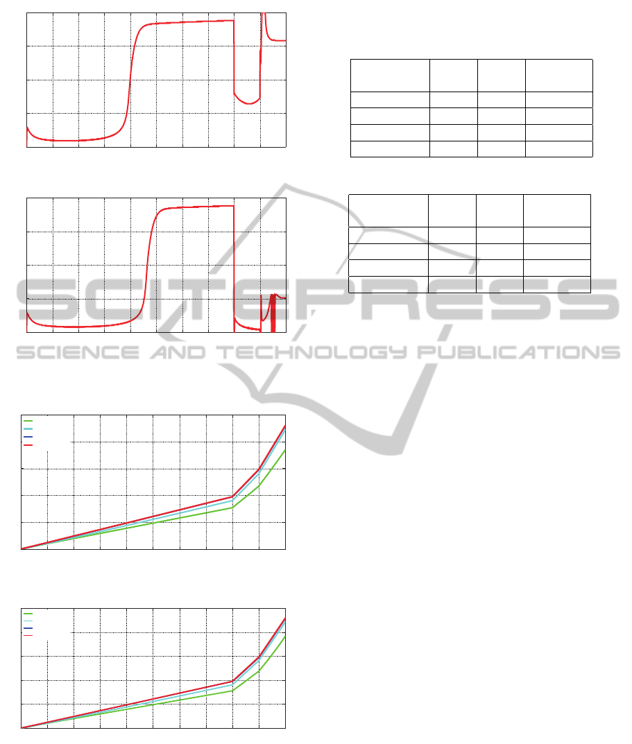
Then, to confirm the acceleration performance, we
compare MP-SMC-I with SMC-I, SMC and No con-
trol. As shown in fig. 7, the curve of the vehicle ve-
locity with MP-SMC-I coincides with the one with
SMC-I almost. But we can see that the vehicle with
MP-SMC-I represented by the red curve achieves the
maximum driving force for the best acceleration dur-
ing the whole simulation time.
Finally, table 3 show the results of the energy con-
sumed E
r
, the total distance D
d
and the energy con-
sumption rate E
p
for different mass of vehicle. We
can see that the energy consumption rate with MP-
ICINCO2015-12thInternationalConferenceonInformaticsinControl,AutomationandRobotics
156
0 1 2 3 4 5 6 7 8 9 10
0
50
100
150
200
Time [s]
K
in
(i) M = 1000[kg]
0 1 2 3 4 5 6 7 8 9 10
0
50
100
150
200
Time [s]
K
in
(ii) M = 1400[kg]
Figure 6: Time response of K
in
for MP-SMC-I).
0 1 2 3 4 5 6 7 8 9 10
0
5
10
15
20
25
Time [s]
Body velocity [m/s]
b
b
No control
SMC
SMC−I
MP−SMC−I
(i) M = 1000[kg]
0 1 2 3 4 5 6 7 8 9 10
0
5
10
15
20
25
Time [s]
Body velocity [m/s]
b
b
No control
SMC
SMC−I
MP−SMC−I
(ii) M = 1400[kg]
Figure 7: Time response of body velocity with No control,
SMC, SMC-I and MP-SMC-I.
SMC-I is nearly as much as the one with SMC-I, but
the total distance is longer than SMC-I. This indicates
that the vehicle with MP-SMC-I achieve a better ac-
celeration performance. As the same result as the pre-
Table 3: Results of energy consumption rate with No con-
trol, SMC, SMC-I and MP-SMC-I.
(i) ( M = 1000[kg])
E
r
D
d
E
p
[Wh] [m] [Wh/km]
No control 80.34 55.52 1447
SMC 28.30 64.82 437
SMC-I 28.11 69.58 404
MP-SMC-I 28.64 70.03 409
(ii) (M = 1400[kg])
E
r
D
d
E
p
[Wh] [m] [Wh/km]
No control 62.75 56.33 1114
SMC 35.10 64.98 540
SMC-I 36.22 69.54 521
MP-SMC-I 36.90 70.02 527
vious chapter described, due to the mass increasing
caused much energy cost that the EV should be made
more light without detriment to performance.
5 CONCLUSIONS
In this paper, the improved MP-SMC-I method has
been proposed for robust slip suppression problem of
EVs. We can verified that the the proposed method
shows good robust performance against the changing
of road condition and vehicle mass by numerical sim-
ulations. Also this method shows the good energy
consumption performance. At the present stage, ef-
fectiveness of the proposed method is only confirmed
by numerical simulations. Next step, therefore, is to
realize the real system using the proposed method
and to proof the advantage of such system by real
experiments. Furthermore, in future work, the suit-
ability of the proposed method must be studied not
only for the slip suppression addressed by this paper
but also for overall driving including during braking.
Even for this issue, however, the basic framework of
the method can be expanded relatively easily to the
foundation for making practical EVs with high per-
formance and safety traction control systems.
ACKNOWLEDGEMENTS
This research was partially supported by Grant-
in-Aid for Scientific Research (C) (Grant number:
24560538; Tohru Kawabe; 2012-2014) from the Min-
istry of Education, Culture, Sports, Science and Tech-
nology of Japan.
AModelPredictiveSlidingModeControlwithIntegralActionforSlipSuppressionofElectricVehicles
157

REFERENCES
Brown, S., Pyke, D., and Steenhof, P. (2010). Electric ve-
hicles: The role and importance of standards in an
emerging market. Energy Policy, 38(7):3797–3806.
Dargay, J., Gately, D., and Sommer, M. (2007). Vehi-
cle ownership and income growth, worldwide: 1960-
2030. The Energy Journal, 28(4):143–170.
Eker, I. and Akinal, A. (2008). Sliding mode control with
integral augmented sliding surface: Design and exper-
imental application to an electromechanical system.
Electrical Engineering, 90:189–197.
Fujii, K. and Fujimoto, H. (2007). Slip ratio control based
on wheel control without detection of vehiclespeed for
electric vehicle. IEEJ Technical Meeting Record, VT-
07-05:27–32.
Hirota, T., Ueda, M., and Futami, T. (2011). Activities
of electric vehicles and prospect for future mobility.
Journal of The Society of Instrument and Control En-
gineering, 50:165–170.
Hori, Y. (2000). Simulation of mfc-based adhesion con-
trol of 4wd electric vehicle. IEEJ Record of Industrial
Measurement and Control, pages IIC–00–12.
Kawabe, T. (2014). Model predictive 2dof pid control for
slip suppression of electric vehicles. Proceedings of
11th International Conference on Informatics in Con-
trol, Automation and Robotics, 2:12–19.
Kawabe, T., Kogure, Y., Nakamura, K., Morikawa, K., and
Arikawa, K. (2011). Traction control of electric vehi-
cle by model predictive pid controller. Transaction of
JSME Series C, 77(781):3375–3385.
Li, S. and Kawabe, T. (2013). Slip suppression of electric
vehicles using sliding mode control method. Interna-
tional Journal of Intelligent Control and Automation,
4(3):327–334.
Li, S. and Kawabe, T. (2014). Slip suppression of elec-
tric vehicles using sliding mode control based on mpc
algorithm. International Journal of Engineering and
Industries, 5(4):11–23.
Maciejowski, J. (2005). Predictive Control with Con-
straints. Tokyo Denki University Press (Trans. by
Adachi,S. and Kanno,M.) (in Japanese).
Mamalis, A., Spentzas, K., and Mamali, A. (2013). The im-
pact of automotive industry and its supply chain to cli-
mate change: Somme techno-economic aspects. Eu-
ropean Transport Research Review, 5(1):1–10.
Pacejka, H. and Bakker, E. (1991). The magic formula tire
model. Vehicle system dynamics, 21:1–18.
Slotine, J. and Li, W. (1991). Applied nonlinear control.
Prentice-Hall.
Tseng, H., Wu, J., and Liu, X. (2013). Affordability of
electric vehicle for a sustainable transport system: An
economic and environmental analysis. Energy Policy,
61:441–447.
ICINCO2015-12thInternationalConferenceonInformaticsinControl,AutomationandRobotics
158
