
Robot Navigation using Velocity Potential Fields and Particle Filters
for Obstacle Avoidance
Dan-Sorin Necsulescu
1
, Jin Bai
1
and Jurek Sasiadek
2
1
Department of Mechanical Engineering, University of Ottawa. Ottawa, Canada
2
Department of Mechanical and Aerospace Engineering, Carleton University, Ottawa, Canada,
Keywords: Autonomous Robot, Particle Filter, Obstacle Avoidance, FastSLAM, Velocity Potential Fields.
Abstract: Autonomous robots are required to avoid the obstacles during navigation. For this purpose unknown and
unexpected obstacles have to be detected during motion. The proposed approach uses particle filters to
process sensors data and estimate relative position of the robot with regard to the obstacles and to the goal.
These relative position estimations are inputs to the velocity potential field approach for obtaining time
varying velocity commands for the robot to avoid all obstacles and reach the goal.
1 INTRODUCTION
Robot motion control needs data about the absolute
position of the goal and the relative positions of the
unexpected obstacles with regards to the robot.
Often, a map of the surrounding area is needed. A
solution to the simultaneous localization and map
building, presented by Dissanayake et al, 2001,
permits an autonomous vehicle to start in an
unknown location in an unknown environment and,
using relative observations only, incrementally build
a map of the world and to compute an estimate of
vehicle location. Montemerlo et al, 2001, paper
presents FastSLAM, an algorithm that recursively
estimates the full posterior distribution over robot
pose and landmark locations which scales
logarithmically with the number of landmarks in the
map. Doucet et al, 2001, proposed sequential Monte
Carlo methods for the case that prior knowledge
about the phenomenon being modelled is available.
This knowledge allows to formulate Bayesian
models, relating prior knowledge with current
observations, often done on-line. Particle filters offer
a very interesting approach for obtaining such a
local map from range sensing (Rekleitis, 2004),
(Arulampalam, 2002, Svensson, 2014). Based on
such maps, robot controllers have to provide
commands for moving toward the goal while
avoiding obstacles. Wang, 2009 proposed a generic
force field method for robot real-time motion
planning based on location, orientation, travel speed,
priority, size, and the robot’s environment. A
dynamic variable speed force field method was
designed for applications in partially known and
dynamically changing environments.
An efficient approach for robot motion control
without the risk of local minima is provided by
velocity potential field approach, (Masoud, 2007). A
fuzzy logic navigation and obstacle avoidance by a
mobile robot in an unknown dynamic environment is
proposed by Faisal et al, 2013.
In this paper a robot motion controller for
obstacles avoidance using particle filter method is
proposed. When the robot detects the obstacles, a
map of local environment can be re-built based on
data received from the sensors of the robot. A novel
approach for robot navigation is achieved using the
integration of particle filter method with velocity
potential field approach.
2 SYSTEM MODEL
The robot we use and its sensing range is shown in
Figure 1, in which we can see that this sensing range
of the robot is divided into three sections, i.e. left
(yellow), right (green) and back (white). Local map
is built with regard to front, left and right sections
which sense obstacles. Since the robot will not move
backwards in our experiments, we do not use back
sections for detecting obstacles. The inner circle is
the safety range; if obstacles lie in this area, the
robot has to turn away in order to avoid them. The
outer circle is the searching range, which shows the
maximum range robot can detect. The blue ellipse in
Figure 1 illustrates the obstacle. θ
k
is the angle
between the heading of the robot and the positive
direction of x axis. β
k
denotes the angle between the
43
Necsulescu D., Bai J. and Sasiadek J..
Robot Navigation using Velocity Potential Fields and Particle Filters for Obstacle Avoidance.
DOI: 10.5220/0005501400430048
In Proceedings of the 12th International Conference on Informatics in Control, Automation and Robotics (ICINCO-2015), pages 43-48
ISBN: 978-989-758-122-9
Copyright
c
2015 SCITEPRESS (Science and Technology Publications, Lda.)

straight line from the robot pointing to the goal and
the positive direction of x axis.
Robots can find the minimum distance to
obstacles with one specific beam. The coordinates of
the intersection point of that beam with obstacles
could be obtained. Based on knowing the position of
the intersection point, two measurements with regard
to that intersection point are enough to determine the
position of the robot accurately; one is the distance
d
min
from the robot to the intersection point and the
other is the angle α between the chosen beam and
the positive direction of x axis, both shown in Figure
1,
We choose these two measurements for the
output vector
min,
,
T
kkk
yd
(1)
where k indicates the measurements taken at time k.
The detected obstacle is treated as a landmark or
beacon in order to get the measurements.
We use the coordinate (at time k) of the robot as
hidden states
,
T
kkk
Xxy
(2)
The state space model is
1
,,
,,
kkkkk
kkkkk
xfxu
y
hxuv
(3)
where u
k
is the control vector of the system and the
noise sequences ω
k
and v
k
are assumed as
independent white noise processes with known
probability density function (pdf). We indicate the
intersection point of the chosen beam and the
obstacle as
**
,
T
kkk
pxy
(4)
Goal
Local Map
Local Map
,
GG
x
y
y
x
0
,,
kkk
xy
min,k
d
k
k
k
k
V
Figure 1: Local map built when sensing obstacles.
Based on the algorithm of obstacle avoidance using
velocity potential field approach (Necsulescu, 2014,
Nie, 2014), we can expand Equation (3) as
22
22
min min
m
max max
1
max max
min min
min
1cos
1sin
11
cos cos
2
1
Gk Gk
goal
Gk Gk
goal
safe safe
xx yy
R
ak
kk
xx yy
R
ak
dd
RR
nkt k
d
n
kv e T
xxT
kv e T
ke ke
dd
ke
d
in min
min
22
1
sin sin
2
arctan
safe safe
k
d
RR
kt k
kk k k
kk
kk
kk
ke
d
xx yy
yv
yy
xx
(5)
In equation (5), T is the time step for robot
control.
a
k
,
n
k
,
t
k
are gains for attractive, normal
repulsive and tangential repulsive velocity,
respectively. d
min
is the minimum detected distance
from the robot to obstacles. R
goal
is the radius of a
region around the goal; when robot enters that
region it will decrease the speed. R
safe
is the radius
with reference to the obstacles, such that when the
distance d
min
from robot to obstacles is less than that
radius, the robot will activate obstacles avoidance
algorithm. v
max
and ω
max
are the maximum velocity
and angular velocity of the robot. Equation (5) is
applied for two situations. First, when d
min
is larger
than R
safe
and, second, when d
min
is less than or
equals to R
safe
. In the first case, Equation (5) is
adapted such that the robot has applied only the
attractive velocity command. In the second case, the
robot is also subject to the repulsive velocity
command.
For the first case, when obstacles are not present
any more, equation (5) is reduced to which gives the
trajectories of the robot to the goal.
22
22
max max
1
max max
22
1cos
1sin
arctan
Gk Gk
goal
Gk Gk
goal
xx yy
R
ak
kk k
xx yy
R
ak
kk kk
kk
kk
kk
kv e T
xxT
kv e T
xx yy
yv
yy
xx
(6)
ICINCO2015-12thInternationalConferenceonInformaticsinControl,AutomationandRobotics
44

For the second case, when obstacles are present,
equation (5) is modified into the following equation
(7).
min
min
min
min
min
1
min
min
min
22
1
cos
1
sin
1
cos
2
1
sin
2
arctan
safe
safe
safe
safe
d
R
nk
kk
d
R
nk
d
R
tk
k
d
R
tk
kk kk
k
kk
kk
ke
d
xxT
ke
d
ke
d
ke
d
xx yy
y
yy
xx
k
v
(7)
Equation (7) contains a command for the robot to
avoid obstacles with the attractive term of Equation
(5) removed as obstacles appear. When dimensions
of left obstacles are larger than right ones, the robot
will turn right in order to save energy and time in
avoiding obstacles, and vice versa. We gauge the
size of obstacles based on the number of intersecting
points of sensor beams and obstacles.
3 PARTICLE FILTERING TO
TRACK THE ROBOT
After modeling the system, next step in simulation is
to produce N initial particles
,
(i=1,…,N) based on
the pdf p(x
0
). Since we already know the initial pose
of the robot, we will produce particles right in the
initial position of the robot.
Then, based on the dynamics equation of
equation set (5), we generate time propagation
values for all particles
,11,11
, , 1,...,
ii
ki k k i k k
x
fxu i N
(8)
to obtain a new set of a priori particles.
Then we compare
,
,
,
with y
k
, i.e. we
evaluate
|
,
, and obtain corresponding
. It
should be observed that since we have two
measurements, the weight
is composed of the
product of two other weights as follows
,,
ii i
kkdk
WW W
(9)
where
,
is the weight obtained based
on
|
,
. We use the normal distribution pdf to
evaluate the weights comparing
,
,
,
with
the measured distance d
min,k
, i.e. y
k
. The more
,
,
,
is closer to d
min,k
, the bigger the
weight of that particle is. Likewise,
,
is the
weight related to
|
,
,
,
,
,
close to
will have allocated a higher weight based on the
pdf of normal distribution. We prefer particles
whose
,
,
,
is close to d
min,k
and
,
respectively, which result in larger
because of
larger
,
and larger
,
. Larger
,
or larger
,
only cannot produce larger
, since accurate
tracking of the robot needs to combine two
parameters (the distance and the angle) together.
Equation (9) results from the need that the particles
satisfy both the required distance and the required
angle.
After obtaining the weights
for all particles
,
(i=1,…,N), they are normalized to obtain a set of
normalized weight s
(i=1,…,N). Until now we
formed a first set of particles
,
,
(i=1,…,N) in
preparation for the next step resampling.
There are lots of resampling methods introduced
in the literature. In this paper we use the method in
Svensson, 2014. These particles
,
after resampling
with the same weight w are going to be propagated
in time based on Equation (8) to arrive to the next
iteration. The same process will be applied to the
particles in next iteration.
The particle filtering for robot path estimation is
applied until there are no measurements left, since
without measurements we cannot get the weight for
each particle. Likewise, if the robot cannot detect an
obstacle in the beginning, the particle filter is still
not able to work because of no measurements. It
would also be possible that the robot can find
obstacles in the beginning, whereas during its
navigation process to the goal there may be some
time when the robot finds no obstacles. At that time
the particle filter is not going to be active until robot
can find obstacles again.
After obtaining a new set of a posteriori particles
though resampling, we can compute any desired
statistical measure of this set of particles. Typically
most interest is in evaluating the mean and the
covariance for all these particles.
When the estimation of robot path is already
known, the estimation of landmark positions
conditioned on the estimated robot path based on the
measurements can be obtained. For each of the
robot’s estimated position, the measurement without
noise is considered, then the estimation of landmark
from the corresponding measurements is obtained.
Each measurement consists of the true measurement
RobotNavigationusingVelocityPotentialFieldsandParticleFiltersforObstacleAvoidance
45
and the noise and we use the true measurement
without noise to better estimate the position of
landmark. If there are several measurements of one
landmark, Kalman filter has to be applied to get
optimal estimation of that landmark based on all
related measurements (Simon, 2006). In our
experiments we assume that each landmark is
reflected in one measurement only in the whole
process, and we do not apply Kalman filter to
landmark estimation.
4 SIMULATION RESULTS FOR
ROBOT NAVIGATION WITH
OBSTACLE AVOIDANCE
In the simulations, we consider robot navigation in
the case of two obstacles with different dimensions
to illustrate the performance of the proposed
algorithm. Our simulation is conducted by using a
switching controller such that the robot will choose
proper turning direction based on the local map it
created.
In the simulation, one can see that the robot
successfully chose a direction that resulted in a
higher efficiency and saved more time in avoiding
obstacles while finally reaching the goal. In the
process, while the robot was travelling towards the
goal, estimations of robot path and positions of
landmarks (obstacles) were obtained.
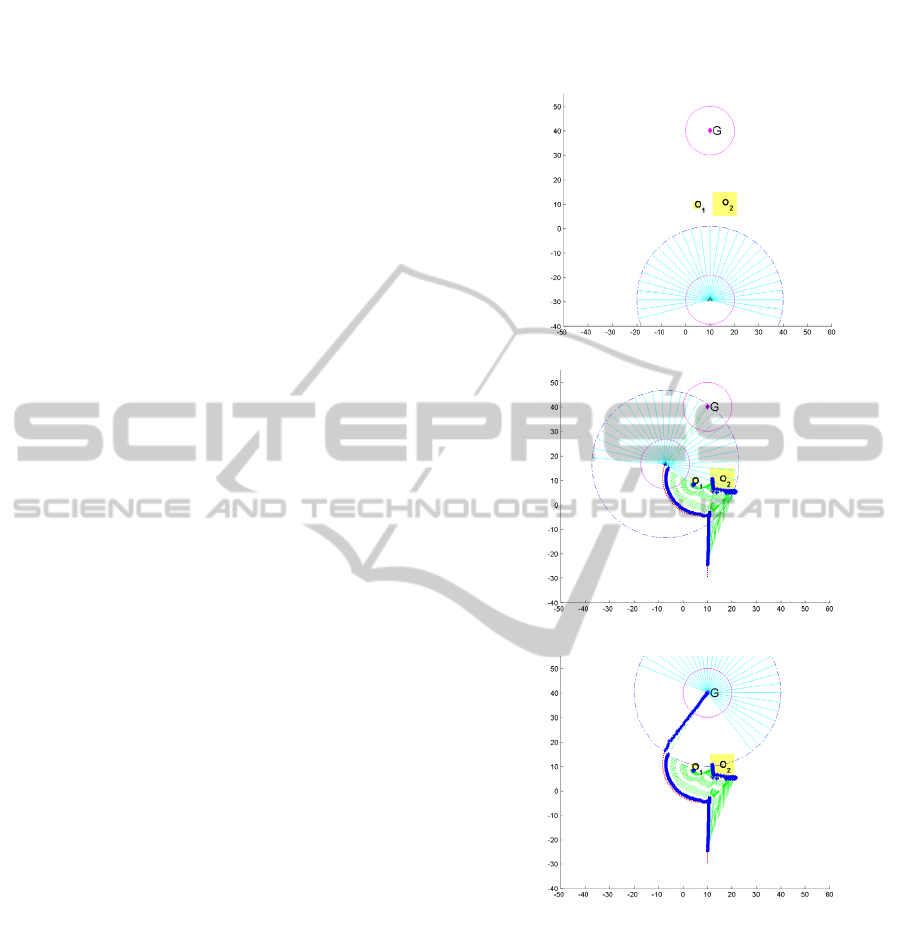
Figure 2 shows robot navigation toward the goal
while avoiding two obstacles of different dimensions
and too close to permit passing in-between.
FastSLAM approach is used to obtain the
estimations of robot path and positions of obstacles.
In this simulation, the robot built a local map finding
that O
2
has larger dimension than O
1
, so that it
turned left when close to the obstacles. At the same
time, the red dotted line indicates the ideal robot
path based on our controller, and the blue square
illustrates the estimated robot path; asterisk signs
around the obstacles indicate the estimated positions
of obstacles. The obstacle avoidance algorithm is
based on the proposed velocity potential fields
approach, and the estimations with regard to robot
path and obstacles are performed by using the
FastSLAM approach.
In Figure 2 several snapshots of robot navigation
are shown. When the robot detected obstacles,
estimations of the robot path used the measurements
with regard to the obstacles. However, when robot
bypassed obstacles and sensed the goal, the
estimation of the robot path is based on
measurements with regard to the goal only. The
estimated robot path and the real robot path
converge finally when robot reaches the goal.
Figure 2: Robot travelling around two obstacles with the
FastSLAM approach.
Symbols used are:
magenta diamond= Goal,
yellow square= Obstacle,
red dotted line= Ideal robot path,
blue square= Estimated robot position wrt obstacles,
blue asterisk= Estimated obstacle position,
blue pentagram=Estimated robot position wrt the
goal,
green dashed line= Estimated measurement line.
X(m)
Y(m)
Y(m)
X(m)
X(m)
Y(m)
ICINCO2015-12thInternationalConferenceonInformaticsinControl,AutomationandRobotics
46
5 EXPERIMENTAL RESULTS –
TWO DIFFERENT OBSTACLES
The experiments were performed using LabVIEW
TM
and MATLAB
TM
. LabVIEW is used to control the
robot reaching the goal without obstacles collision,
and collect data regarding the measurements about
obstacles and the goal. The measurement data is
composed of distance measurement between the
robot and obstacles/the goal and angle measurement
between the chosen beam and the positive direction
of x axis. After getting the measurement data, we
utilized MATLAB to build the estimated map and
the estimated robot path based on data we collected.
In the experiment, we consider the same scenario
used in the simulation, in which the robot has to
avoid two obstacles with different dimensions. The
experiments with a robot travelling around two
obstacles will be illustrated in two parts. The first
part is related to robot navigation with two obstacles
avoidance using the velocity potential field
approach. During this navigation process, we
collected sensor data for each robot moving step and
recorded them. Robot trajectory is composed of a
large number of small steps. Due to the accuracy of
the rotation sensor imbedded in the servo motor, we
recorded the sensor data every π/8 of sensor rotation.
In the second part of our experiment the
estimations of robot path and obstacles are obtained
based on the sensor data collected in order to build
the local map, obtained using MATLAB.
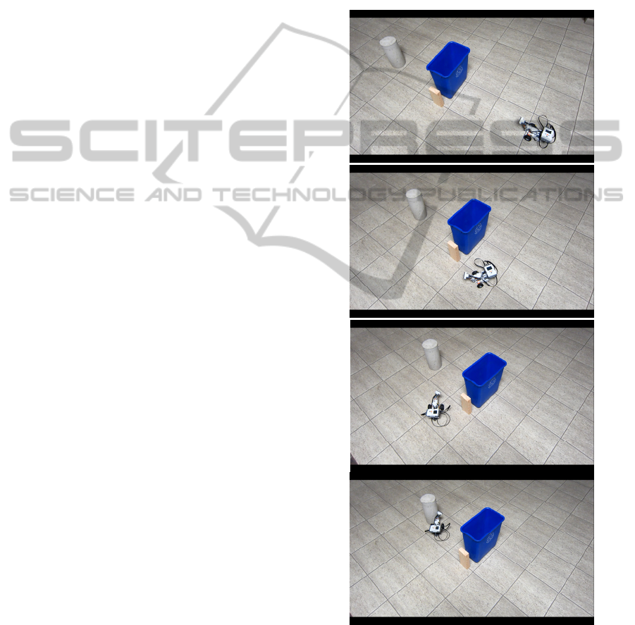
In Figure 3, the grey cylinder in the left top corner of
the snapshot indicates the robot goal. Between the
robot and the goal are two obstacles, a blue trash bin
with a bigger size than the small obstacle, a wood
block..
Several snapshots are shown in Figure 3. The
robot controller chooses proper direction to turn in
order to save time and energy. We can see that the
controller successfully drove the robot while
avoiding obstacles to reach the goal. The results in
Figure 3 also show the choice of turning left, a
proper turning direction given obstacles dimensions.
Sensor data were collected in the robot
navigation process. Based on the data collected, a
map was built using the estimations of robot
positions and the local map robot sensed, as shown
in Figure 4.
In Figure 4, the magenta circle indicates the goal.
The red solid line indicates the ideal robot path to
the goal without obstacles collision, the green square
denotes the estimation with regard to obstacles
sensed by the robot, and the green diamond
illustrates the estimation with regard to the goal. The
green asterisk sign refers to the local map robot built
based on the sensor data. We can see that, when
robot detects the goal, the estimation of robot
position performs better than that based on the
measurements with regard to obstacles given the
absolute position of the goal in the global map is
known. Given that obstacle O
2
is bigger than O
1
the
robot controller chose to turn left to avoid collision.
The particle clouds representation of Figure 4 is
shown in Figure 5.
Figure 3: Robot navigation with two obstacles avoidance
reaching the goal.
RobotNavigationusingVelocityPotentialFieldsandParticleFiltersforObstacleAvoidance
47
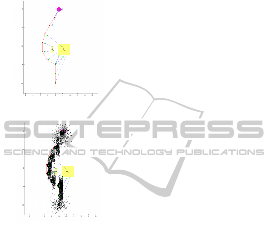
Figure 4: Estimations of robot positions and two obstacles.
Figure 5: Particle clouds representation of Figure 4.
6 CONCLUSIONS
A novel combination of velocity potential field
approach for motion control with a particle filter for
unknown obstacles localization proved a good
solution for obstacle avoidance without reching a
local minimum. An improvement of the velocity
potential field approach is included to select proper
direction of robot turning in front of obstacles.
Simulation and experimental results verified the
proposed approach for
the case of obstacles
positioned in-between initial robot position and goal
position.
For future, much more complex scenarios
could be investigated, such as moving obstacles or
humans, in order to test the validity of the proposed
approach.
REFERENCES
Arulampalam, M. S., Maskell, S., Gordon, N. & Clapp, T.,
2002. A tutorial on particle filters for online
nonlinear/non-gaussian Bayesian tracking, IEEE
Transactions on Signal Processing, 50(2), pp.174-188.
Dissanayake, G., Newman, P., Clark, S., Durrant-Whyte,
H. F., Csorba, M. 2001. A solution to the
simultaneous. localization and map building (SLAM)
problem. IEEE. Transactions of Robotics and
Automation. Vol 17 , Issue 3, pp. 229 – 241.
Doucet, A., de Freitas, N., Gordon, N., 2001. An.
Introduction to Sequential Monte Carlo Methods,
Sequential Monte Carlo Methods in Practice, pp 3-14.
Faisal, M., Hedjar, R., Sulaiman, M. A., Al-Mutib, K.,
2013. Fuzzy Logic Navigation and Obstacle
Avoidance by a Mobile Robot in an Unknown
Dynamic Environment, International Journal of
Advanced Robotic Systems, Vol. 10, pp.1-7.
Masoud, A., 2007, “Decentralized self-organizing
potential field-based control for individually motivated
mobile agents in a cluttered environment: A vector-
harmonic potential field”. IEEE Transactions on
Systems, Man and Cybernetics, Part A: Systems and
Humans, 37(3), pp. 372-390.
Montemerlo, M., Thrun, M. Koller, D. and Wegbreit, B.
2001. “FastSLAM: A Factored Solution to the.
Simultaneous Localization and Mapping Problem”
AAAI Proceedings. pp. 593-598.
Necsulescu, D., G. Nie, 2014, Quasi-harmonic Approach.
to Non- holonomic Robot Motion Control with.
Concave Obstacles Avoidance, 2014CCDC Conf.,
Changsa, China, May 31 - June 2.
Nie, G, 2014. Quasi-Harmonic Function Approach to
Human-Following Robots, M. S. thesis, Dept. of
Mechanical Engineering, Univ. Ottawa, Ottawa, ON.
Rekleitis, I. M., 2004, A Particle Filter Tutorial for Mobile
Robot Localization, Center for Intelligent Machines,
McGill University, Report TR-CIM-04-02.
Simon, D., 2006. Optimal State Estimation: Kalman, H
Infinity, and Nonlinear Approaches, Hoboken, N. J.
Wiley-Interscience.
Wang, D., 2009. A Generic Force Field Method for Robot.
Real-time Motion Planning and Coordination. PhD
dissertation, University of Technology, Sydney,
Australia.
Svensson, A., 2014, An introduction to particle filters,
Department of Information Technology, Uppsala
University, Uppsala, Sweden.
X(m)
Y(m)
X(m)
Y(m)
ICINCO2015-12thInternationalConferenceonInformaticsinControl,AutomationandRobotics
48
