Data Fusion Between a 2D Laser Profile Sensor and a Camera
M. Wagner
1
, P. Heß
1
, S. Reitelsh
¨
ofer
2
and J. Franke
2
1
Nuremberg Campus of Technology, Nuremberg Institute of Technology, F
¨
urther Straße 246c, 90429, Nuremberg, Germany
2
Institute for Factory Automation and Production Systems, Friedrich-Alexander-Universit
¨
at Erlangen-N
¨
urnberg, Germany
Keywords:
3D Reconstruction, Calibration, Color Extension, Sensor Data Fusion, Workpiece Scanning.
Abstract:
This paper describes a color extension of a 2D laser profile sensor by extracting the corresponding color from a
camera image. For these purpose, we developed a routine for an extrinsic calibration between the profile sensor
and the camera. Based on the resulting translation and rotation vectors a belonging pixel can be calculated
for each profile point. Consequently, the color for each profile point can be extracted from the image. This
approach is used to extend the geometric data of a robotic based 3D scanning system by color data.
1 INTRODUCTION
The range of applications for industrial robots ex-
tends. Especially small and medium-sized enterprises
focus on small quantities and consequently a high
flexibility. Thus, workpiece related robot program-
ming is used with increasing frequency for typical
robotic tasks, such as handling, processing or inspec-
tion. In most cases, an already existing CAD-model
is used for this purpose, but for some applications the
scanning of individual workpieces can be necessary.
This is a fast way to get an accurate 3D model of the
real workpiece, especially from unknown objects.
Laser scanners are commonly used for the scan-
ning of workpieces. They are very efficient in extract-
ing geometric information, but one main drawback of
laser sensors is their lack of capability in capturing
textures of objects. Thus, common 2D laser profile
sensors do not have color information implied. In
this paper, we present an extension of a common 2D
laser profile sensor with color information by extract-
ing them from a camera image. One possible way to
fuse the data is to detect the laser profile in the image
and fit it to the measured profile, but the visibility of
the laser depends strongly on the color and the sur-
face of the scanned object. In addition, it means a lot
expenditure to fit the profiles. The selected approach
avoids these disadvantages, by fusing the data of the
two sensors through the transformation between the
base coordinate systems. Thereby, the position of the
profile points in the image can be calculated regard-
less of the visibility of the laser.
To find correspondences between the points of the
profile sensor and the pixels of the camera image the
geometric transformation between the sensor frames
needs to be determined by a calibration. First, an in-
trinsic calibration of the used camera is done for this
purpose. The second calibration step is the extrinsic
calibration between the profile sensor and the camera.
Based on the resulting calibration parameters, a cal-
culation of the corresponding pixels can be realized.
Finally, the color is determined from the image.
The subsequent content of this paper is structured
as follows. The related work in the field of extrin-
sic calibrations between a camera and a laser scanner
is presented in the following section. Furthermore,
the approaches for the sensor calibration and the color
extraction are described in detail. The fourth section
deals with the accuracy investigation of the realized
approach. A short conclusion is at the end of the pa-
per.
2 RELATED WORK
The consideration of the related work is separated
in two sections. Initially, a short summary of 3D
workpieces scanning through industrial robot arms is
given. The state of the art in sensor fusion between
laser scanners and cameras follows afterwards.
2.1 Robot-based Workpiece Scanning
The reconstruction of 3D shapes can be done with
a multitude of sensors and approaches. Thus, many
contact or non-contact sensors, such as radiation-,
159
Wagner M., Heß P., Reitelshöfer S. and Franke J..
Data Fusion Between a 2D Laser Profile Sensor and a Camera.
DOI: 10.5220/0005501601590165
In Proceedings of the 12th International Conference on Informatics in Control, Automation and Robotics (ICINCO-2015), pages 159-165
ISBN: 978-989-758-123-6
Copyright
c
 2015 SCITEPRESS (Science and Technology Publications, Lda.)

light- or image-based sensors, are on the market–
either they are three-dimensional sensors or they are
one- or two-dimensional sensors moved by hand or by
machine. One flexible machine for doing this motion
is an industrial robot arm. By linking the measure-
ment points with the robot positions, 3D point data
can be derived.
For robotic based workpiece scanning non-contact
sensors are mainly used. Due to the requirement for
a high accuracy and a close range triangulation-based
sensors are preferred. Thus, 2D laser profile sensors
are frequently used for scanning workpieces by mov-
ing the sensor by a robot arm (Larsson and Kjellan-
der, 2006; Borangiu and Dumitrache, 2010; Li et al.,
2011; Shen and Zhu, 2012). These scanning sys-
tems for example are used for a reverse engineering
process, as shown in (Larsson and Kjellander, 2006).
A workpiece scanning for subsequent processing has
been pursued in (Borangiu and Dumitrache, 2010).
Most of the approaches use an additional rotation ta-
ble on which the workpiece is placed to improve the
reachability. In our approach, the system is extended
by moving the workpiece with a second robot arm (cf.
Figure 1) to improve the reachability furthermore and
to include the robot-related workpiece position in the
scans for following processing steps.
The realized scans with all of these robotic-based
systems include only the geometric information, what
is sufficient for many applications. No color informa-
tion is included, but for example for object recogni-
tion or realistic model building it can be necessary.
Therefore, they need to be obtained by additional sen-
sors.
2.2 Sensor Fusion
Not for every application a perfect individual sensor
is available. Thus, multiple sensors need to be used
frequently to achieve all of the necessary data. To
combine the data of multiple sensors an extrinsic cal-
Camera Scanner
Gripper Workpiece
Figure 1: Robot set-up for workpiece scanning.
ibration between the sensor coordinate systems must
be done first. Therefore, related reference points visi-
ble in all of the data sets need to be obtained.
Many approaches for the fusion of a camera and a
2D or 3D laser scanner have been realized in the past.
The main application is navigation for mobile robots
(Zhang and Pless, 2004; Mei and Rives, 2006; Scara-
muzza et al., 2007; G. Li et al., 2009; Nunez et al.,
2009) or vehicles (Garcia-Alegre et al., 2011; Osgood
and Huang, 2013). Object recognition–also for mo-
bile robots (Klimentjew et al., 2010) or vehicles (Mo-
hottala et al., 2009)–is a frequent application, too. In
addition, other applications, for example model build-
ing or medical applications, are considered (Cobzas
et al., 2002).
Some of the realized extrinsic calibration methods
use manually selected reference points, as shown in
(Cobzas et al., 2002) or in (Scaramuzza et al., 2007).
More intuitive approaches use calibration objects for
an automatic reference point detection. Approaches
with known and with unknown objects are realized.
Most of them use a calibration plane to detect refer-
ences. Thus, for example in (Zhang and Pless, 2004)
and in (Mohottala et al., 2009) a checkerboard in dif-
ferent poses has been used. The approach realized in
(G. Li et al., 2009) uses the edges of a plane and in
(Nunez et al., 2009) only the corners of a rectangu-
lar object, such as a pattern, are used. Another way
is the use of patterns with geometrical extensions, as
shown in (Klimentjew et al., 2010). In this approach,
a typically checkered pattern is extended with a 3D
structure to get reference points in both data sets. The
corners or walls of a room can be used as well (Mei
and Rives, 2006). Some approaches use specific sin-
gle objects as reference points. Thus, in (Osgood and
Huang, 2013) small white discs are placed in the laser
plane and detected through the reflection in the cam-
era image, for example. In (Navarrete et al., 2013)
small catadioptrics are used and the laser intensity in-
formation is converted to a 2D image which is fused
with the camera image.
To the best of our knowledge, no approach for a
color extension of a short ranged 2D laser profile sen-
sor has been realized, yet.
3 APPROACH
The color extension of the robotic-based 3D scanning
system is based on the data fusion between the geo-
metric position data from the profile sensor and the
belonging color data from the camera image. This
process is done in four main steps (cf. Figure 2).
ICINCO2015-12thInternationalConferenceonInformaticsinControl,AutomationandRobotics
160

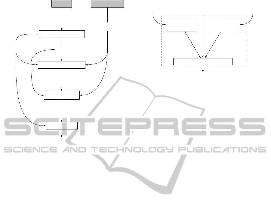
Camera
Profile sensor
Intrinsic calibration
Extrinsic calibration
Calculat pixels
Extract color
Color values
Rectified image
Profile points
A, k
Raw image
r, t
Pixels
Figure 2: Color extension routine.
First, the used sensors need to be calibrated intrin-
sic to ensure the accuracy of the measurements. The
used profile sensor is already calibrated by the manu-
facturer. Thus, only the camera needs to be calibrated
intrinsic to achieve a rectified image. The resulting
intrinsic camera parameters and the rectified image is
used for the following extrinsic calibration between
the camera and the profile sensor by getting matched
image and profile points. The extrinsic calibration
results the transformation between the two sensors.
With the intrinsic and the extrinsic parameters a be-
longing pixel can be calculated for each profile point.
In the last step, for each profile point a color is ex-
tracted from the rectified image.
The main steps of the color extension routine are
described in the following subsections in detail.
3.1 Intrinsic Calibration
Before the fusion of the two sensors data, each of
the sensors need to be calibrated intrinsic. As al-
ready mentioned before, the used 2D laser profile sen-
sor is already calibrated intrinsic by the manufacturer.
Therefore, this step does not need to be considered.
However, this does not apply for the camera.
As already shown by (Tan et al., 1995), classic
camera calibration methods use complicated calibra-
tion objects, with known 3D coordinates. Newer cali-
bration methods either seek calibration cues from the
scene or only require simple calibration objects. A
common method is the calibration by a planar pat-
Rectified
images
Profile
points
A, k
r, t
Image
processing
Profile
processing
Transformation calculation
Image
reference
points
Profile
reference
points
Figure 3: Extrinsic calibration routine.
tern published in (Zhang, 2000). By moving either
the camera or the pattern and detecting the pattern in
the image in multiple poses, the intrinsic parameters
can be calculated. They consist of the intrinsic matrix
A =



f
x
γ c
x
0 f
y
c
y
0 0 1



and the distortion vector k = (k
1
k
2
p
1
p
2
)
T
. We use
this approach with a typical 9 × 6 chessboard. The
implementation is based on the open source library
OpenCV.
3.2 Extrinsic Calibration
The realized extrinsic calibration routine is shown in
Figure 3. Before calculating the transformation be-
tween the sensors, each sensor data is processed to
achieve the reference points. Afterwards, the trans-
lation vector t = (t
x
t
y
t
z
)
T
and the rotation vector
r = (θ
x
θ
y
θ
z
)
T
are calculated from the reference
points and the intrinsic camera parameters.
In our approach, any planar calibration object fit-
ting in the measurement range of the profile sensor is
usable. The exact color and size of the object is not
important. As reference points the corner points of
the profile and the end points of the laser line inside
of the image are detected.
3.2.1 Profile Processing
Starting from the fact that only the calibration ob-
ject is in the range of the profile sensor, we achieve
the profile reference points by taking the two profile
points with the smallest and the largest x-value.
To make sure that all reference points are mea-
sured correctly, the trapezium shaped measuring
range is limited as follows (cf. Figure 4). First, the
values are limited to a z-range, that is a little bit (e.g.
DataFusionBetweena2DLaserProfileSensorandaCamera
161

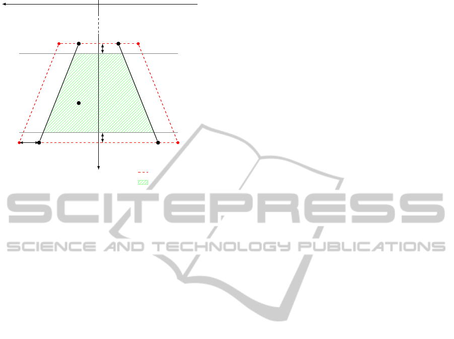
x
z
P
P
min
P
N
min
P
P
max
P
N
max
z
min
z
max
P
n
Sensor range
Measurement range
∆z
∆z
∆x
Figure 4: Range limitation for the profile sensor.
five times the z-resolution) smaller than the z-range of
the sensor, to ensure that no reference points close to
the boundary of the sensor-range are taken. Thus, the
z-range borders are shifted about ∆z and only points
inside of these borders are used furthermore. In the
next step, the x-value of the reference points is con-
trolled by calculating the two scalar products:
d
P
= (P
P
max
− P
P
min
) ·(P
n
− P
P
max
) (1)
d
N
= (P
N
min
− P
N
max
) · (P
n
− P
N
min
) (2)
Thereby, the sensor range is reduced on both sides
about ∆x. If d
P
> 0 and d
N
> 0, the reference point
P
n
is inside of the limited range and can be used for
calibration. A calibration object close to or even out-
side of the profile sensor measurement range results
negative values. Thus, these points are not saved for
calibration.
3.2.2 Image Processing
The laser appears in a visible line on the calibration
object. The visibility of the laser depends on the mate-
rial and the surface of the scanned object as well as the
viewing angle. Therefore, we reduce the camera im-
age to a binary image with values that are in range of
a color spectrum matching to the laser line color. The
spectrum is selected individually by choosing ranges
either for the HSV (hue-saturation-value) or the RGB
(Red-Green-Blue) parameters. Furthermore, an ero-
sion and a dilation is done on the binary image to
clearly stand out the laser line. In the next step, a line
fitting procedure using least squares method is done,
resulting the linear equation. The two end points of
the line are achieved by determining the bounding box
and calculating the points of intersection between the
box and the linear equation.
To ensure that all image reference points are col-
lected correctly, the image frame is also reduced by a
small stripe. Thus, only points inside of the reduced
frame are accepted. If the calibration object is posi-
tioned close or even outside of the image frame, no
reference points are saved.
3.2.3 Transformation Calculation
The transformation between the profile sensor and
the camera consists of translations in the three di-
mensions and rotations around the three axis, repre-
sented by a translation vector t and a rotation vec-
tor r. The calculation of the transformation between
the two sensor coordinate systems is done by an it-
erative method based on Levenberg-Marquardt opti-
mization. This method has already successfully been
used in several previous approaches for sensor fusion
(Cobzas et al., 2002; Zhang and Pless, 2004; Scara-
muzza et al., 2007; Mohottala et al., 2009). In order
to solve the established equation systems N ≥ 3 refer-
ence points are necessary. Since we have two points
per measurement, at least two measurements are re-
quired. From the N corresponding reference points in
the profile P
Re f
n
and in the image I
Re f
n
as well as the
intrinsic camera parameters A and k (cf. Section 3.1)
the translation t and the rotation r finally result.
3.3 Pixel Calculation
Both used sensors only offer two-dimensional infor-
mation. Thus, the profile points P
n
= (p
x
0 p
z
)
T
and
the image points I
n
= (i
x
i
y
0)
T
contain only two vari-
ables. The relationship between the data points can be
described by the following equation:
I
n
(i
x
, i
y
) = R · P
n
(p
x
, p
z
) + t (3)
Using this geometric relation, a belonging pixel
for every profile point could be calculated. The ro-
tation matrix R can be derived from rotation r de-
termined through the extrinsic calibration (cf. Sec-
tion 3.2) as well as the translation t. The resulting
pixel corresponds the projection of the profile point
onto the image plane.
3.4 Color Extraction
Several approaches are possible for the extraction of
the color values from the camera image. The most
obvious one is the extraction directly from the calcu-
lated pixels. However, with visible laser sensors the
ICINCO2015-12thInternationalConferenceonInformaticsinControl,AutomationandRobotics
162

object is discolored by the laser in these areas. Thus,
the laser needs to be turned of temporary, for exam-
ple through pulsation. But this takes time, which is
disadvantageous especially in a full 3D scan. This
drawback can be avoided by coloring the entire point
cloud after the scan. Therefore, multiple images could
be necessary to color all sides of the point cloud. But
in this case, the color information is not already us-
able during the individual profile shots. Our third ap-
proach avoids both disadvantages by approximately
determining the color values from neighboring pix-
els. For this purpose, for each profile point two neigh-
bor points N
n
= (p
x
± δ p
z
)
T
with a distance δ in y-
direction are used to calculate the corresponding pix-
els by:
I
n
(i
x
, i
y
) = R · N
n
(p
x
, ±δ, p
z
) + t (4)
The offset must be chosen large enough that the
laser is not hit anymore. The corresponding color
value is then averaged from the color values of the two
nearby pixels. Thus, the color values can be quickly
obtained on-the-fly, with the disadvantage of an inac-
curacy.
4 EXPERIMENTS AND RESULTS
As mentioned in Section 3.2, any planar calibra-
tion object fitting in the measurement range of the
profile sensor is usable for our approach. As ex-
ample we use Lego bricks with different colors
in order to investigate the influence of the color
(cf. Figure 5). The used camera is a Logitech
920c with a resolution of 1920 × 1080 and a frame
rate of 30 fps. The used laser profile sensor is
a Micro-Epsilon scanCONTROL 2600-100 with a
range from 125.0 mm to 390.0 mm in z-direction.
The x-range of the sensor is between ±28.5 mm and
ScannerCamera
Calibration
object
Figure 5: Experimental set-up for sensor fusion.
H
S
V
Figure 6: Exemplar color spectrum (H : 339
◦
− 351
◦
,
S : 29.8 − 87.2 %, V : 98.0 − 100.0 %) for line detection.
±71.0 mm. Inside of this range the sensor is mea-
suring 640 points per profile with a z-resolution of
12 µm. Through the adjustable shutter time the sen-
sor can be set well to different surfaces.
For the individual color of the calibration object
a specific color spectrum is selected through a color
dialog or through a pipette, by clicking on to image
pixels. Thus, one of the lightest pixels and one of the
darkest pixels of the laser line is selected to achieve a
good spectrum. An example spectrum is depicted in
Figure 6.
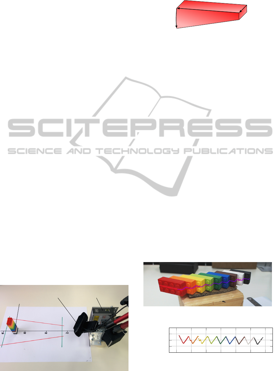
To illustrate the correctness of the calibration,
stepped Lego bricks with different colors along the
profile are used, as shown in Figure 7. The profile
point based calculated pixels are colored purple in-
side of this image. It becomes apparent, that the cal-
culated points are close to the actual laser line. Based
on the calculated pixels the color information is ex-
tracted from the camera image and the corresponding
color profile is visualized in Figure 8, showing the
color changes at step transitions.
In order to make a concrete statement about the ac-
curacy of the calibration, the belonging pixel for each
profile reference point and furthermore the distance
between the pixel and the corresponding end of the
detected line is calculated. From the sum of the dis-
tances of all used reference points the average pixel
error is calculated.
Twenty calibrations with two experimental set-ups
Figure 7: Multi-color example for color extraction.
−60
−40 −20 0 20 40
60
250
255
260
265
270
−60
−40 −20 0 20 40
60
250
255
260
265
270
−60
−40 −20 0 20 40
60
250
255
260
265
270
−60
−40 −20 0 20 40
60
250
255
260
265
270
−60
−40 −20 0 20 40
60
250
255
260
265
270
−60
−40 −20 0 20 40
60
250
255
260
265
270
−60
−40 −20 0 20 40
60
250
255
260
265
270
−60
−40 −20 0 20 40
60
250
255
260
265
270
−60
−40 −20 0 20 40
60
250
255
260
265
270
−60
−40 −20 0 20 40
60
250
255
260
265
270
−60
−40 −20 0 20 40
60
250
255
260
265
270
−60
−40 −20 0 20 40
60
250
255
260
265
270
−60
−40 −20 0 20 40
60
250
255
260
265
270
−60
−40 −20 0 20 40
60
250
255
260
265
270
−60
−40 −20 0 20 40
60
250
255
260
265
270
−60
−40 −20 0 20 40
60
250
255
260
265
270
−60
−40 −20 0 20 40
60
250
255
260
265
270
−60
−40 −20 0 20 40
60
250
255
260
265
270
−60
−40 −20 0 20 40
60
250
255
260
265
270
−60
−40 −20 0 20 40
60
250
255
260
265
270
−60
−40 −20 0 20 40
60
250
255
260
265
270
−60
−40 −20 0 20 40
60
250
255
260
265
270
−60
−40 −20 0 20 40
60
250
255
260
265
270
−60
−40 −20 0 20 40
60
250
255
260
265
270
−60
−40 −20 0 20 40
60
250
255
260
265
270
−60
−40 −20 0 20 40
60
250
255
260
265
270
−60
−40 −20 0 20 40
60
250
255
260
265
270
−60
−40 −20 0 20 40
60
250
255
260
265
270
−60
−40 −20 0 20 40
60
250
255
260
265
270
−60
−40 −20 0 20 40
60
250
255
260
265
270
−60
−40 −20 0 20 40
60
250
255
260
265
270
−60
−40 −20 0 20 40
60
250
255
260
265
270
−60
−40 −20 0 20 40
60
250
255
260
265
270
−60
−40 −20 0 20 40
60
250
255
260
265
270
−60
−40 −20 0 20 40
60
250
255
260
265
270
−60
−40 −20 0 20 40
60
250
255
260
265
270
−60
−40 −20 0 20 40
60
250
255
260
265
270
−60
−40 −20 0 20 40
60
250
255
260
265
270
−60
−40 −20 0 20 40
60
250
255
260
265
270
−60
−40 −20 0 20 40
60
250
255
260
265
270
−60
−40 −20 0 20 40
60
250
255
260
265
270
−60
−40 −20 0 20 40
60
250
255
260
265
270
−60
−40 −20 0 20 40
60
250
255
260
265
270
−60
−40 −20 0 20 40
60
250
255
260
265
270
−60
−40 −20 0 20 40
60
250
255
260
265
270
−60
−40 −20 0 20 40
60
250
255
260
265
270
−60
−40 −20 0 20 40
60
250
255
260
265
270
−60
−40 −20 0 20 40
60
250
255
260
265
270
−60
−40 −20 0 20 40
60
250
255
260
265
270
−60
−40 −20 0 20 40
60
250
255
260
265
270
−60
−40 −20 0 20 40
60
250
255
260
265
270
−60
−40 −20 0 20 40
60
250
255
260
265
270
−60
−40 −20 0 20 40
60
250
255
260
265
270
−60
−40 −20 0 20 40
60
250
255
260
265
270
−60
−40 −20 0 20 40
60
250
255
260
265
270
−60
−40 −20 0 20 40
60
250
255
260
265
270
−60
−40 −20 0 20 40
60
250
255
260
265
270
−60
−40 −20 0 20 40
60
250
255
260
265
270
−60
−40 −20 0 20 40
60
250
255
260
265
270
−60
−40 −20 0 20 40
60
250
255
260
265
270
−60
−40 −20 0 20 40
60
250
255
260
265
270
−60
−40 −20 0 20 40
60
250
255
260
265
270
−60
−40 −20 0 20 40
60
250
255
260
265
270
−60
−40 −20 0 20 40
60
250
255
260
265
270
−60
−40 −20 0 20 40
60
250
255
260
265
270
−60
−40 −20 0 20 40
60
250
255
260
265
270
−60
−40 −20 0 20 40
60
250
255
260
265
270
−60
−40 −20 0 20 40
60
250
255
260
265
270
−60
−40 −20 0 20 40
60
250
255
260
265
270
−60
−40 −20 0 20 40
60
250
255
260
265
270
−60
−40 −20 0 20 40
60
250
255
260
265
270
−60
−40 −20 0 20 40
60
250
255
260
265
270
−60
−40 −20 0 20 40
60
250
255
260
265
270
−60
−40 −20 0 20 40
60
250
255
260
265
270
−60
−40 −20 0 20 40
60
250
255
260
265
270
−60
−40 −20 0 20 40
60
250
255
260
265
270
−60
−40 −20 0 20 40
60
250
255
260
265
270
−60
−40 −20 0 20 40
60
250
255
260
265
270
−60
−40 −20 0 20 40
60
250
255
260
265
270
−60
−40 −20 0 20 40
60
250
255
260
265
270
−60
−40 −20 0 20 40
60
250
255
260
265
270
−60
−40 −20 0 20 40
60
250
255
260
265
270
−60
−40 −20 0 20 40
60
250
255
260
265
270
−60
−40 −20 0 20 40
60
250
255
260
265
270
−60
−40 −20 0 20 40
60
250
255
260
265
270
−60
−40 −20 0 20 40
60
250
255
260
265
270
−60
−40 −20 0 20 40
60
250
255
260
265
270
−60
−40 −20 0 20 40
60
250
255
260
265
270
−60
−40 −20 0 20 40
60
250
255
260
265
270
−60
−40 −20 0 20 40
60
250
255
260
265
270
−60
−40 −20 0 20 40
60
250
255
260
265
270
−60
−40 −20 0 20 40
60
250
255
260
265
270
−60
−40 −20 0 20 40
60
250
255
260
265
270
−60
−40 −20 0 20 40
60
250
255
260
265
270
−60
−40 −20 0 20 40
60
250
255
260
265
270
−60
−40 −20 0 20 40
60
250
255
260
265
270
−60
−40 −20 0 20 40
60
250
255
260
265
270
−60
−40 −20 0 20 40
60
250
255
260
265
270
−60
−40 −20 0 20 40
60
250
255
260
265
270
−60
−40 −20 0 20 40
60
250
255
260
265
270
−60
−40 −20 0 20 40
60
250
255
260
265
270
−60
−40 −20 0 20 40
60
250
255
260
265
270
−60
−40 −20 0 20 40
60
250
255
260
265
270
−60
−40 −20 0 20 40
60
250
255
260
265
270
−60
−40 −20 0 20 40
60
250
255
260
265
270
−60
−40 −20 0 20 40
60
250
255
260
265
270
−60
−40 −20 0 20 40
60
250
255
260
265
270
−60
−40 −20 0 20 40
60
250
255
260
265
270
−60
−40 −20 0 20 40
60
250
255
260
265
270
−60
−40 −20 0 20 40
60
250
255
260
265
270
−60
−40 −20 0 20 40
60
250
255
260
265
270
−60
−40 −20 0 20 40
60
250
255
260
265
270
−60
−40 −20 0 20 40
60
250
255
260
265
270
−60
−40 −20 0 20 40
60
250
255
260
265
270
−60
−40 −20 0 20 40
60
250
255
260
265
270
−60
−40 −20 0 20 40
60
250
255
260
265
270
−60
−40 −20 0 20 40
60
250
255
260
265
270
−60
−40 −20 0 20 40
60
250
255
260
265
270
−60
−40 −20 0 20 40
60
250
255
260
265
270
−60
−40 −20 0 20 40
60
250
255
260
265
270
−60
−40 −20 0 20 40
60
250
255
260
265
270
−60
−40 −20 0 20 40
60
250
255
260
265
270
−60
−40 −20 0 20 40
60
250
255
260
265
270
−60
−40 −20 0 20 40
60
250
255
260
265
270
−60
−40 −20 0 20 40
60
250
255
260
265
270
−60
−40 −20 0 20 40
60
250
255
260
265
270
−60
−40 −20 0 20 40
60
250
255
260
265
270
−60
−40 −20 0 20 40
60
250
255
260
265
270
−60
−40 −20 0 20 40
60
250
255
260
265
270
−60
−40 −20 0 20 40
60
250
255
260
265
270
−60
−40 −20 0 20 40
60
250
255
260
265
270
−60
−40 −20 0 20 40
60
250
255
260
265
270
−60
−40 −20 0 20 40
60
250
255
260
265
270
−60
−40 −20 0 20 40
60
250
255
260
265
270
−60
−40 −20 0 20 40
60
250
255
260
265
270
−60
−40 −20 0 20 40
60
250
255
260
265
270
−60
−40 −20 0 20 40
60
250
255
260
265
270
−60
−40 −20 0 20 40
60
250
255
260
265
270
−60
−40 −20 0 20 40
60
250
255
260
265
270
−60
−40 −20 0 20 40
60
250
255
260
265
270
−60
−40 −20 0 20 40
60
250
255
260
265
270
−60
−40 −20 0 20 40
60
250
255
260
265
270
−60
−40 −20 0 20 40
60
250
255
260
265
270
−60
−40 −20 0 20 40
60
250
255
260
265
270
−60
−40 −20 0 20 40
60
250
255
260
265
270
−60
−40 −20 0 20 40
60
250
255
260
265
270
−60
−40 −20 0 20 40
60
250
255
260
265
270
−60
−40 −20 0 20 40
60
250
255
260
265
270
−60
−40 −20 0 20 40
60
250
255
260
265
270
−60
−40 −20 0 20 40
60
250
255
260
265
270
−60
−40 −20 0 20 40
60
250
255
260
265
270
−60
−40 −20 0 20 40
60
250
255
260
265
270
−60
−40 −20 0 20 40
60
250
255
260
265
270
−60
−40 −20 0 20 40
60
250
255
260
265
270
−60
−40 −20 0 20 40
60
250
255
260
265
270
−60
−40 −20 0 20 40
60
250
255
260
265
270
−60
−40 −20 0 20 40
60
250
255
260
265
270
−60
−40 −20 0 20 40
60
250
255
260
265
270
−60
−40 −20 0 20 40
60
250
255
260
265
270
−60
−40 −20 0 20 40
60
250
255
260
265
270
−60
−40 −20 0 20 40
60
250
255
260
265
270
−60
−40 −20 0 20 40
60
250
255
260
265
270
−60
−40 −20 0 20 40
60
250
255
260
265
270
−60
−40 −20 0 20 40
60
250
255
260
265
270
−60
−40 −20 0 20 40
60
250
255
260
265
270
−60
−40 −20 0 20 40
60
250
255
260
265
270
−60
−40 −20 0 20 40
60
250
255
260
265
270
−60
−40 −20 0 20 40
60
250
255
260
265
270
−60
−40 −20 0 20 40
60
250
255
260
265
270
−60
−40 −20 0 20 40
60
250
255
260
265
270
−60
−40 −20 0 20 40
60
250
255
260
265
270
−60
−40 −20 0 20 40
60
250
255
260
265
270
−60
−40 −20 0 20 40
60
250
255
260
265
270
−60
−40 −20 0 20 40
60
250
255
260
265
270
−60
−40 −20 0 20 40
60
250
255
260
265
270
−60
−40 −20 0 20 40
60
250
255
260
265
270
−60
−40 −20 0 20 40
60
250
255
260
265
270
−60
−40 −20 0 20 40
60
250
255
260
265
270
−60
−40 −20 0 20 40
60
250
255
260
265
270
−60
−40 −20 0 20 40
60
250
255
260
265
270
−60
−40 −20 0 20 40
60
250
255
260
265
270
−60
−40 −20 0 20 40
60
250
255
260
265
270
−60
−40 −20 0 20 40
60
250
255
260
265
270
−60
−40 −20 0 20 40
60
250
255
260
265
270
−60
−40 −20 0 20 40
60
250
255
260
265
270
−60
−40 −20 0 20 40
60
250
255
260
265
270
−60
−40 −20 0 20 40
60
250
255
260
265
270
−60
−40 −20 0 20 40
60
250
255
260
265
270
−60
−40 −20 0 20 40
60
250
255
260
265
270
−60
−40 −20 0 20 40
60
250
255
260
265
270
−60
−40 −20 0 20 40
60
250
255
260
265
270
−60
−40 −20 0 20 40
60
250
255
260
265
270
−60
−40 −20 0 20 40
60
250
255
260
265
270
−60
−40 −20 0 20 40
60
250
255
260
265
270
−60
−40 −20 0 20 40
60
250
255
260
265
270
−60
−40 −20 0 20 40
60
250
255
260
265
270
−60
−40 −20 0 20 40
60
250
255
260
265
270
−60
−40 −20 0 20 40
60
250
255
260
265
270
−60
−40 −20 0 20 40
60
250
255
260
265
270
−60
−40 −20 0 20 40
60
250
255
260
265
270
−60
−40 −20 0 20 40
60
250
255
260
265
270
−60
−40 −20 0 20 40
60
250
255
260
265
270
−60
−40 −20 0 20 40
60
250
255
260
265
270
−60
−40 −20 0 20 40
60
250
255
260
265
270
−60
−40 −20 0 20 40
60
250
255
260
265
270
−60
−40 −20 0 20 40
60
250
255
260
265
270
−60
−40 −20 0 20 40
60
250
255
260
265
270
−60
−40 −20 0 20 40
60
250
255
260
265
270
−60
−40 −20 0 20 40
60
250
255
260
265
270
−60
−40 −20 0 20 40
60
250
255
260
265
270
−60
−40 −20 0 20 40
60
250
255
260
265
270
−60
−40 −20 0 20 40
60
250
255
260
265
270
−60
−40 −20 0 20 40
60
250
255
260
265
270
−60
−40 −20 0 20 40
60
250
255
260
265
270
−60
−40 −20 0 20 40
60
250
255
260
265
270
−60
−40 −20 0 20 40
60
250
255
260
265
270
−60
−40 −20 0 20 40
60
250
255
260
265
270
−60
−40 −20 0 20 40
60
250
255
260
265
270
−60
−40 −20 0 20 40
60
250
255
260
265
270
−60
−40 −20 0 20 40
60
250
255
260
265
270
−60
−40 −20 0 20 40
60
250
255
260
265
270
−60
−40 −20 0 20 40
60
250
255
260
265
270
−60
−40 −20 0 20 40
60
250
255
260
265
270
−60
−40 −20 0 20 40
60
250
255
260
265
270
−60
−40 −20 0 20 40
60
250
255
260
265
270
−60
−40 −20 0 20 40
60
250
255
260
265
270
−60
−40 −20 0 20 40
60
250
255
260
265
270
−60
−40 −20 0 20 40
60
250
255
260
265
270
−60
−40 −20 0 20 40
60
250
255
260
265
270
−60
−40 −20 0 20 40
60
250
255
260
265
270
−60
−40 −20 0 20 40
60
250
255
260
265
270
−60
−40 −20 0 20 40
60
250
255
260
265
270
−60
−40 −20 0 20 40
60
250
255
260
265
270
−60
−40 −20 0 20 40
60
250
255
260
265
270
−60
−40 −20 0 20 40
60
250
255
260
265
270
−60
−40 −20 0 20 40
60
250
255
260
265
270
−60
−40 −20 0 20 40
60
250
255
260
265
270
−60
−40 −20 0 20 40
60
250
255
260
265
270
−60
−40 −20 0 20 40
60
250
255
260
265
270
−60
−40 −20 0 20 40
60
250
255
260
265
270
−60
−40 −20 0 20 40
60
250
255
260
265
270
−60
−40 −20 0 20 40
60
250
255
260
265
270
−60
−40 −20 0 20 40
60
250
255
260
265
270
−60
−40 −20 0 20 40
60
250
255
260
265
270
−60
−40 −20 0 20 40
60
250
255
260
265
270
−60
−40 −20 0 20 40
60
250
255
260
265
270
−60
−40 −20 0 20 40
60
250
255
260
265
270
−60
−40 −20 0 20 40
60
250
255
260
265
270
−60
−40 −20 0 20 40
60
250
255
260
265
270
−60
−40 −20 0 20 40
60
250
255
260
265
270
−60
−40 −20 0 20 40
60
250
255
260
265
270
−60
−40 −20 0 20 40
60
250
255
260
265
270
−60
−40 −20 0 20 40
60
250
255
260
265
270
−60
−40 −20 0 20 40
60
250
255
260
265
270
−60
−40 −20 0 20 40
60
250
255
260
265
270
−60
−40 −20 0 20 40
60
250
255
260
265
270
−60
−40 −20 0 20 40
60
250
255
260
265
270
−60
−40 −20 0 20 40
60
250
255
260
265
270
−60
−40 −20 0 20 40
60
250
255
260
265
270
−60
−40 −20 0 20 40
60
250
255
260
265
270
−60
−40 −20 0 20 40
60
250
255
260
265
270
−60
−40 −20 0 20 40
60
250
255
260
265
270
−60
−40 −20 0 20 40
60
250
255
260
265
270
−60
−40 −20 0 20 40
60
250
255
260
265
270
−60
−40 −20 0 20 40
60
250
255
260
265
270
−60
−40 −20 0 20 40
60
250
255
260
265
270
−60
−40 −20 0 20 40
60
250
255
260
265
270
−60
−40 −20 0 20 40
60
250
255
260
265
270
−60
−40 −20 0 20 40
60
250
255
260
265
270
−60
−40 −20 0 20 40
60
250
255
260
265
270
−60
−40 −20 0 20 40
60
250
255
260
265
270
−60
−40 −20 0 20 40
60
250
255
260
265
270
−60
−40 −20 0 20 40
60
250
255
260
265
270
−60
−40 −20 0 20 40
60
250
255
260
265
270
−60
−40 −20 0 20 40
60
250
255
260
265
270
−60
−40 −20 0 20 40
60
250
255
260
265
270
−60
−40 −20 0 20 40
60
250
255
260
265
270
−60
−40 −20 0 20 40
60
250
255
260
265
270
−60
−40 −20 0 20 40
60
250
255
260
265
270
−60
−40 −20 0 20 40
60
250
255
260
265
270
−60
−40 −20 0 20 40
60
250
255
260
265
270
−60
−40 −20 0 20 40
60
250
255
260
265
270
−60
−40 −20 0 20 40
60
250
255
260
265
270
−60
−40 −20 0 20 40
60
250
255
260
265
270
−60
−40 −20 0 20 40
60
250
255
260
265
270
−60
−40 −20 0 20 40
60
250
255
260
265
270
−60
−40 −20 0 20 40
60
250
255
260
265
270
−60
−40 −20 0 20 40
60
250
255
260
265
270
−60
−40 −20 0 20 40
60
250
255
260
265
270
−60
−40 −20 0 20 40
60
250
255
260
265
270
−60
−40 −20 0 20 40
60
250
255
260
265
270
−60
−40 −20 0 20 40
60
250
255
260
265
270
−60
−40 −20 0 20 40
60
250
255
260
265
270
−60
−40 −20 0 20 40
60
250
255
260
265
270
−60
−40 −20 0 20 40
60
250
255
260
265
270
−60
−40 −20 0 20 40
60
250
255
260
265
270
−60
−40 −20 0 20 40
60
250
255
260
265
270
−60
−40 −20 0 20 40
60
250
255
260
265
270
−60
−40 −20 0 20 40
60
250
255
260
265
270
−60
−40 −20 0 20 40
60
250
255
260
265
270
−60
−40 −20 0 20 40
60
250
255
260
265
270
−60
−40 −20 0 20 40
60
250
255
260
265
270
−60
−40 −20 0 20 40
60
250
255
260
265
270
−60
−40 −20 0 20 40
60
250
255
260
265
270
−60
−40 −20 0 20 40
60
250
255
260
265
270
−60
−40 −20 0 20 40
60
250
255
260
265
270
−60
−40 −20 0 20 40
60
250
255
260
265
270
−60
−40 −20 0 20 40
60
250
255
260
265
270
−60
−40 −20 0 20 40
60
250
255
260
265
270
−60
−40 −20 0 20 40
60
250
255
260
265
270
−60
−40 −20 0 20 40
60
250
255
260
265
270
−60
−40 −20 0 20 40
60
250
255
260
265
270
−60
−40 −20 0 20 40
60
250
255
260
265
270
−60
−40 −20 0 20 40
60
250
255
260
265
270
−60
−40 −20 0 20 40
60
250
255
260
265
270
x (mm)
z (mm)
x (mm)
z (mm)
x (mm)
z (mm)
x (mm)
z (mm)
x (mm)
z (mm)
x (mm)
z (mm)
x (mm)
z (mm)
x (mm)
z (mm)
x (mm)
z (mm)
x (mm)
z (mm)
x (mm)
z (mm)
x (mm)
z (mm)
x (mm)
z (mm)
x (mm)
z (mm)
x (mm)
z (mm)
x (mm)
z (mm)
x (mm)
z (mm)
x (mm)
z (mm)
x (mm)
z (mm)
x (mm)
z (mm)
x (mm)
z (mm)
x (mm)
z (mm)
x (mm)
z (mm)
x (mm)
z (mm)
x (mm)
z (mm)
x (mm)
z (mm)
x (mm)
z (mm)
x (mm)
z (mm)
x (mm)
z (mm)
x (mm)
z (mm)
x (mm)
z (mm)
x (mm)
z (mm)
x (mm)
z (mm)
x (mm)
z (mm)
x (mm)
z (mm)
x (mm)
z (mm)
x (mm)
z (mm)
x (mm)
z (mm)
x (mm)
z (mm)
x (mm)
z (mm)
x (mm)
z (mm)
x (mm)
z (mm)
x (mm)
z (mm)
x (mm)
z (mm)
x (mm)
z (mm)
x (mm)
z (mm)
x (mm)
z (mm)
x (mm)
z (mm)
x (mm)
z (mm)
x (mm)
z (mm)
x (mm)
z (mm)
x (mm)
z (mm)
x (mm)
z (mm)
x (mm)
z (mm)
x (mm)
z (mm)
x (mm)
z (mm)
x (mm)
z (mm)
x (mm)
z (mm)
x (mm)
z (mm)
x (mm)
z (mm)
x (mm)
z (mm)
x (mm)
z (mm)
x (mm)
z (mm)
x (mm)
z (mm)
x (mm)
z (mm)
x (mm)
z (mm)
x (mm)
z (mm)
x (mm)
z (mm)
x (mm)
z (mm)
x (mm)
z (mm)
x (mm)
z (mm)
x (mm)
z (mm)
x (mm)
z (mm)
x (mm)
z (mm)
x (mm)
z (mm)
x (mm)
z (mm)
x (mm)
z (mm)
x (mm)
z (mm)
x (mm)
z (mm)
x (mm)
z (mm)
x (mm)
z (mm)
x (mm)
z (mm)
x (mm)
z (mm)
x (mm)
z (mm)
x (mm)
z (mm)
x (mm)
z (mm)
x (mm)
z (mm)
x (mm)
z (mm)
x (mm)
z (mm)
x (mm)
z (mm)
x (mm)
z (mm)
x (mm)
z (mm)
x (mm)
z (mm)
x (mm)
z (mm)
x (mm)
z (mm)
x (mm)
z (mm)
x (mm)
z (mm)
x (mm)
z (mm)
x (mm)
z (mm)
x (mm)
z (mm)
x (mm)
z (mm)
x (mm)
z (mm)
x (mm)
z (mm)
x (mm)
z (mm)
x (mm)
z (mm)
x (mm)
z (mm)
x (mm)
z (mm)
x (mm)
z (mm)
x (mm)
z (mm)
x (mm)
z (mm)
x (mm)
z (mm)
x (mm)
z (mm)
x (mm)
z (mm)
x (mm)
z (mm)
x (mm)
z (mm)
x (mm)
z (mm)
x (mm)
z (mm)
x (mm)
z (mm)
x (mm)
z (mm)
x (mm)
z (mm)
x (mm)
z (mm)
x (mm)
z (mm)
x (mm)
z (mm)
x (mm)
z (mm)
x (mm)
z (mm)
x (mm)
z (mm)
x (mm)
z (mm)
x (mm)
z (mm)
x (mm)
z (mm)
x (mm)
z (mm)
x (mm)
z (mm)
x (mm)
z (mm)
x (mm)
z (mm)
x (mm)
z (mm)
x (mm)
z (mm)
x (mm)
z (mm)
x (mm)
z (mm)
x (mm)
z (mm)
x (mm)
z (mm)
x (mm)
z (mm)
x (mm)
z (mm)
x (mm)
z (mm)
x (mm)
z (mm)
x (mm)
z (mm)
x (mm)
z (mm)
x (mm)
z (mm)
x (mm)
z (mm)
x (mm)
z (mm)
x (mm)
z (mm)
x (mm)
z (mm)
x (mm)
z (mm)
x (mm)
z (mm)
x (mm)
z (mm)
x (mm)
z (mm)
x (mm)
z (mm)
x (mm)
z (mm)
x (mm)
z (mm)
x (mm)
z (mm)
x (mm)
z (mm)
x (mm)
z (mm)
x (mm)
z (mm)
x (mm)
z (mm)
x (mm)
z (mm)
x (mm)
z (mm)
x (mm)
z (mm)
x (mm)
z (mm)
x (mm)
z (mm)
x (mm)
z (mm)
x (mm)
z (mm)
x (mm)
z (mm)
x (mm)
z (mm)
x (mm)
z (mm)
x (mm)
z (mm)
x (mm)
z (mm)
x (mm)
z (mm)
x (mm)
z (mm)
x (mm)
z (mm)
x (mm)
z (mm)
x (mm)
z (mm)
x (mm)
z (mm)
x (mm)
z (mm)
x (mm)
z (mm)
x (mm)
z (mm)
x (mm)
z (mm)
x (mm)
z (mm)
x (mm)
z (mm)
x (mm)
z (mm)
x (mm)
z (mm)
x (mm)
z (mm)
x (mm)
z (mm)
x (mm)
z (mm)
x (mm)
z (mm)
x (mm)
z (mm)
x (mm)
z (mm)
x (mm)
z (mm)
x (mm)
z (mm)
x (mm)
z (mm)
x (mm)
z (mm)
x (mm)
z (mm)
x (mm)
z (mm)
x (mm)
z (mm)
x (mm)
z (mm)
x (mm)
z (mm)
x (mm)
z (mm)
x (mm)
z (mm)
x (mm)
z (mm)
x (mm)
z (mm)
x (mm)
z (mm)
x (mm)
z (mm)
x (mm)
z (mm)
x (mm)
z (mm)
x (mm)
z (mm)
x (mm)
z (mm)
x (mm)
z (mm)
x (mm)
z (mm)
x (mm)
z (mm)
x (mm)
z (mm)
x (mm)
z (mm)
x (mm)
z (mm)
x (mm)
z (mm)
x (mm)
z (mm)
x (mm)
z (mm)
x (mm)
z (mm)
x (mm)
z (mm)
x (mm)
z (mm)
x (mm)
z (mm)
x (mm)
z (mm)
x (mm)
z (mm)
x (mm)
z (mm)
x (mm)
z (mm)
x (mm)
z (mm)
x (mm)
z (mm)
x (mm)
z (mm)
x (mm)
z (mm)
x (mm)
z (mm)
x (mm)
z (mm)
x (mm)
z (mm)
x (mm)
z (mm)
x (mm)
z (mm)
x (mm)
z (mm)
x (mm)
z (mm)
x (mm)
z (mm)
x (mm)
z (mm)
x (mm)
z (mm)
x (mm)
z (mm)
x (mm)
z (mm)
x (mm)
z (mm)
x (mm)
z (mm)
x (mm)
z (mm)
x (mm)
z (mm)
x (mm)
z (mm)
x (mm)
z (mm)
x (mm)
z (mm)
x (mm)
z (mm)
x (mm)
z (mm)
x (mm)
z (mm)
x (mm)
z (mm)
x (mm)
z (mm)
x (mm)
z (mm)
x (mm)
z (mm)
x (mm)
z (mm)
x (mm)
z (mm)
x (mm)
z (mm)
x (mm)
z (mm)
x (mm)
z (mm)
x (mm)
z (mm)
x (mm)
z (mm)
x (mm)
z (mm)
x (mm)
z (mm)
x (mm)
z (mm)
x (mm)
z (mm)
x (mm)
z (mm)
x (mm)
z (mm)
x (mm)
z (mm)
x (mm)
z (mm)
x (mm)
z (mm)
x (mm)
z (mm)
x (mm)
z (mm)
x (mm)
z (mm)
x (mm)
z (mm)
x (mm)
z (mm)
x (mm)
z (mm)
x (mm)
z (mm)
x (mm)
z (mm)
x (mm)
z (mm)
x (mm)
z (mm)
x (mm)
z (mm)
x (mm)
z (mm)
x (mm)
z (mm)
x (mm)
z (mm)
x (mm)
z (mm)
x (mm)
z (mm)
x (mm)
z (mm)
x (mm)
z (mm)
x (mm)
z (mm)
x (mm)
z (mm)
x (mm)
z (mm)
x (mm)
z (mm)
x (mm)
z (mm)
x (mm)
z (mm)
x (mm)
z (mm)
x (mm)
z (mm)
x (mm)
z (mm)
x (mm)
z (mm)
x (mm)
z (mm)
x (mm)
z (mm)
x (mm)
z (mm)
x (mm)
z (mm)
x (mm)
z (mm)
x (mm)
z (mm)
x (mm)
z (mm)
x (mm)
z (mm)
x (mm)
z (mm)
x (mm)
z (mm)
x (mm)
z (mm)
Figure 8: Resluting colored profile for Multi-color example.
DataFusionBetweena2DLaserProfileSensorandaCamera
163

have been performed. The first set-up is shown in Fig-
ure 5 and in the second set-up the camera is mounted
as close as possible to the profile sensor. Thereby, ei-
ther two, five or ten object positions scattered inside
of the reference areas were used. However, an in-
creased number of reference points has no significant
influence on the results. Thus, a number of N = 4 ref-
erence points is sufficient. The resulting mean values
and the standard deviation values for each parameter
are shown in Table 1 and 2.
Table 1: Parameter estimation for first experimental
set-up.
t (mm) σ (mm) r (deg) σ (deg) Error (pixel) σ (pixel)
72.3995 0.8716 34.4061 0.1101
80.1886 0.3726 -22.9854 0.2741 0.9349 0.1891
20.5744 0.4808 -3.4034 0.1325
Table 2: Parameter estimation for second experimen-
tal set-up.
t (mm) σ (mm) r (deg) σ (deg) Error (pixel) σ (pixel)
1.9726 0.0445 -9.2074 0.0310
-32.7163 0.1503 -5.9926 0.0370 0.8696 0.0721
-18.5722 0.3498 -89.2548 0.0621
The realized approach achieves stable solutions
and consequently a good repeatability. The validation
shows low standard deviation values for the transfor-
mations (σ < 1mm, σ < 0.3
◦
). A good absolute accu-
racy is also achieved with average pixel errors below
the resolution of the camera (1 pixel). This error oc-
curs partially by rounding errors that can hardly be
avoided.
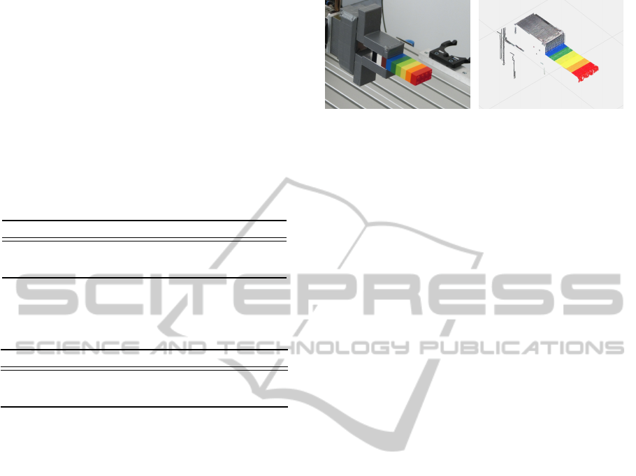
The calibrated sensors are used for workpiece
scanning with two robot arms (cf. Section 2.1). Fig-
ure 9 shows a partial reconstruction of some Lego
bricks held up by a gripper. Due to the contained color
information, it can be clearly distinguished between
the individual bricks and the gripper.
5 CONCLUSIONS
In this paper, a color extension for a 2D laser profile
sensor by getting the color information from a cam-
era is presented. For this purpose, a sensor fusion be-
tween the two sensors has been realized. Therefore,
a flexible calibration routine has been created. Indefi-
nite planar calibration objects are usable with this ap-
proach regardless of their color. The accuracy of the
approach is confirmed through experiments. A pixel
error close to the resolution of the camera has been
achieved.
(a) Scene (b) Point cloud
Figure 9: Example for a colored reconstruction.
So far, the coloring needs approximately 4 ms per
profile point. Future work will be focused on the time
optimization of the process. In addition, an improve-
ment of the reference point distribution, by splitting
the profile sensor measurement range in sections and
a partial restriction on one reference point per section,
is prospected.
REFERENCES
Borangiu, T. and Dumitrache, A. (2010). Robot arms with
3d vision capabilities. In Advances in Robot Manipu-
lator, Vukovar, Croatia. InTech.
Cobzas, D., Zhang, H., and Jagersand, M. (2002). A
comparative analysis of geometric and image-based
volumetric and intensity data registration algorithms.
In Proceedings of the International Conference on
Robotics and Automation, volume 3, Washington, DC,
USA. IEEE.
G. Li, L. D., Pan, L., and Henghai, F. (2009). The cali-
bration algorithm of a 3d color measurement system
based on the line feature.
Garcia-Alegre, M. C., Martin, D., Guinea, D. M., and
Guinea, D. (2011). Real-time fusion of visual images
and laser data images for safe navigation in outdoor
environments. In Sensor Fusion - Foundation and Ap-
plications, Vukovar, Croatia. InTech.
Klimentjew, D., Hendrich, N., and Zhang, J. (2010). Multi
sensor fusion of camera and 3d laser range finder for
object recognition. In Proceedings of the Conference
on Multisensor Fusion and Integration for Intelligent
Systems, Salt Lake City, UT, USA. IEEE.
Larsson, S. and Kjellander, J. (2006). Motion control and
data capturing for laser scanning with an industrial
robot. In Robotics and Autonomous Systems, vol-
ume 54, Amsterdam, Netherlands. Elsevier B.V.
Li, J., Chen, M., Jin, X., Xuebi, C., Yu, D., Z.Dai, Ou, Z.,
and Tang, Q. (2011). Calibration of a multiple axes 3-
d laser scanning system consisting of robot, portable
laser scanner and turntable. In Optik - International
Journal for Light and Electron Optics, volume 122,
Amsterdam, Netherlands. Elsevier B.V.
Mei, C. and Rives, P. (2006). Calibration between a cen-
tral catadioptric camera and a laser range finder for
robotic applications. In Proceedings of the Interna-
tional Conference on Robotics and Automation, Or-
lando, FL, USA. IEEE.
ICINCO2015-12thInternationalConferenceonInformaticsinControl,AutomationandRobotics
164

Mohottala, S., Ono, S., M.Kagesawa, and Ikeuchi, K.
(2009). Fusion of a camera and a laser range sensor for
vehicle recognition. In Proceedings of the Computer
Society Conference on Computer Vision and Pattern
Recognition Workshops, Miami, FL, USA. IEEE.
Navarrete, J., Viejo, D., and Cazorla, M. (2013). Portable
3d laser-camera calibration system with color fusion
for slam. volume 3, Taipei, Taiwan. AUSMT.
Nunez, P., Drews, P., Rocha, R., and Dias, J. (2009). Data
fusion calibration for a 3d laser range finder and a
camera using inertial data. In Proceedings of the 4th
European Conference on Mobile Robots, Barcelona,
Spain. IEEE.
Osgood, T. J. and Huang, Y. (2013). Calibration of laser
scanner and camera fusion system for intelligent vehi-
cles using neldermead optimization. volume 24. IOP
Publishing Ltd.
Scaramuzza, D., Harati, A., and Siegwart, R. (2007). Ex-
trinsic self calibration of a camera and a 3d laser range
finder from natural scenes. In Proceedings of the In-
ternational Conference on Intelligent Robots and Sys-
tems, San Diego, CA, USA. IEEE.
Shen, C. and Zhu, S. (2012). A robotic system for sur-
face measurement via 3d laser scanner. In Proceed-
ings of the 2nd International Conference on Computer
Application and System Modeling, volume 21, Paris,
France. Atlantis Press.
Tan, T. N., Sullivan, G. D., and Baker, K. D. (1995). Recov-
ery of intrinsic and extrinsic camera parameters us-
ing perspective views of rectangles. In Proceedings of
the 1995 British Conference on Machine Vision (Vol.
1), BMVC ’95, pages 177–186, Surrey, UK. BMVA
Press.
Zhang, Q. and Pless, R. (2004). Extrinsic calibration of a
camera and laser range finder (improves camera cal-
ibration). In Proceedings of the International Con-
ference on Intelligent Robots and Systems, volume 3,
Sendai, Japan. IEEE.
Zhang, Z. (2000). A flexible new technique for camera cal-
ibration. IEEE Transactions on Pattern Analysis and
Machine Intelligence, 22(11):1330–1334.
DataFusionBetweena2DLaserProfileSensorandaCamera
165