
Flatness based Feed-forward Control of a Flexible Robot Arm under
Gravity and Joint Friction
Elisha Didam Markus
Department of Electrical, Electronic and Computer Engineering, Central University of Technology, Free State, South Africa
Keywords:
Flexible Joint Robot, Differential Flatness, Trajectory Planning, Friction Control, Open Loop Control.
Abstract:
This paper discusses the open loop control problem of a flexible joint robot that is oriented in the vertical
plane. This orientation of the robot arm introduces gravity constraints and imposes undesirable nonlinear
behavior. Friction is also added at the joints to increase the accuracy of the model. Including these dynamics
to the robot arm amplifies the open loop control problem. Differential flatness is used to propose a feed-
forward control that compensates for these nonlinearities and is able to smoothly steer the robot from rest to
rest positions. The proposed control is achieved without solving any differential equations which makes the
approach computationally attractive. Simulations show the effectiveness of the open loop control design on a
single link flexible joint robot arm.
1 INTRODUCTION
Flexible robots are applied in situations where speed,
dexterity and maneuverability are required. Most
research done in flexible joint robots do not take
unwanted gravitational and frictional effects of the
model into consideration (Kandroodi et al., 2012;
Pereira et al., 2007; Markus et al., 2012b; Jiang
and Higaki, 2011; Tokhi and Azad, 2008; Markus
et al., 2012a; Ozgoli and Taghirad, 2006; Ider and
zgren, 2000; Rodriguez et al., 2014). This is because
the flexible robot at its joint already has a complex
structure (Dwivedy and Eberhard, 2006; Kandroodi
et al., 2012). Firstly, they are underactuated (non-
holonomic)as they possess one control input with two
outputs. Secondly, flexible joint robots are nonmini-
mum phase systems. This is due to the effect of the
link deflection whose movements acts in opposition
to the motor response (Tokhi and Azad, 2008). This
structure already poses problems in the design of their
control. Therefore additional effects of gravity and
friction which are nonlinear dynamics that improve
the accuracy of the model based control are often cir-
cumvented because of their complicated control re-
quirements (Palli et al., 2009; Cambera et al., 2014).
In practice, the effectscannot be completely neglected
or ignored if accurate control is to be achieved.
This study hereby proposes an open loop control
technique for a single link robot under gravity, with
flexibility and friction at the joints. The feedforward
control is useful in applications where fast point to
point movements of the robot are required as is the
case with flexible robots. These type of robot move-
ments tend to induce vibrations at the elastic joints.
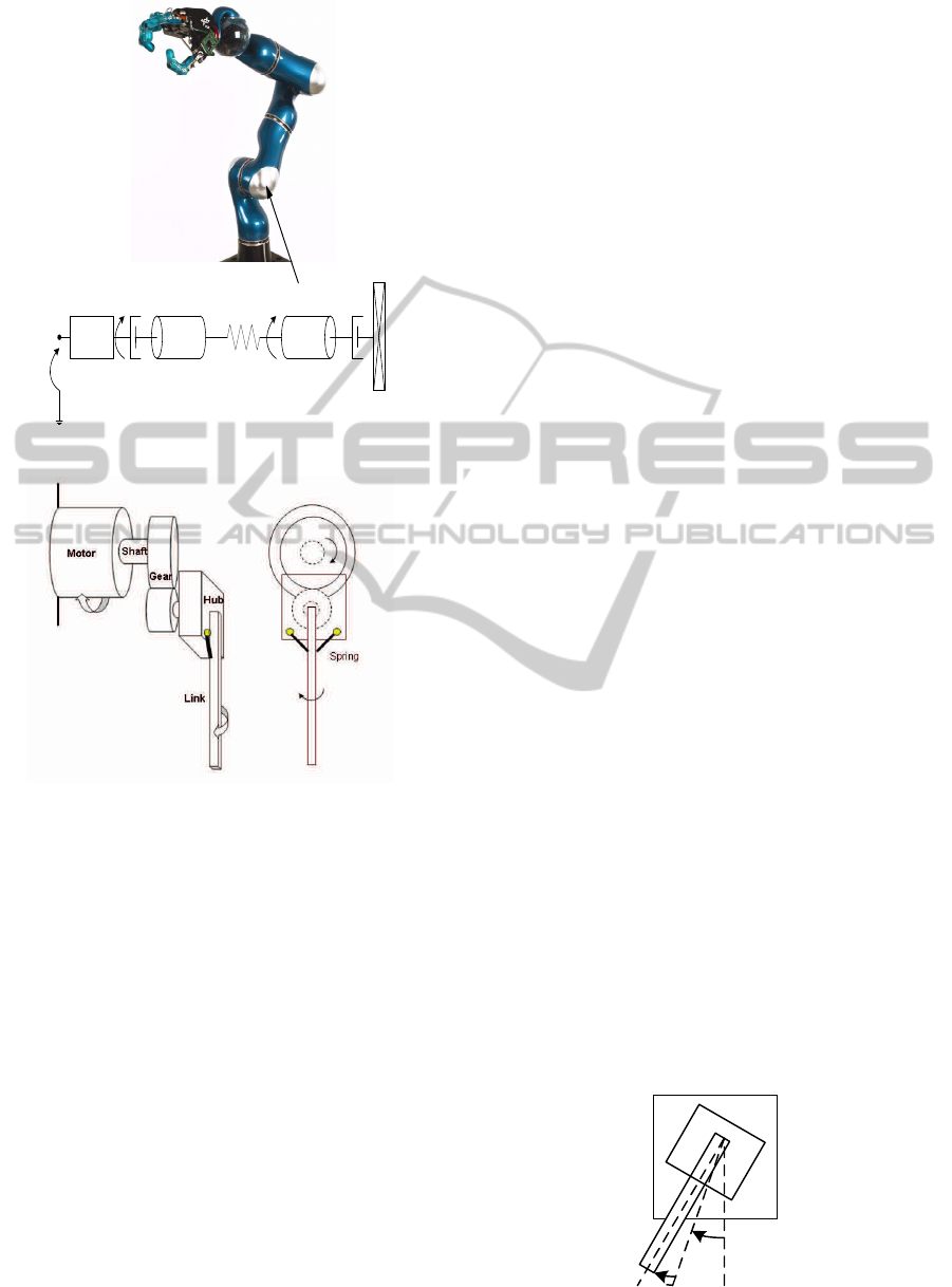
This is common with industrial robots as shown in
figure 1. In order to obtain fast and precise point to
point motion at the joint, the vibrations have to be
compensated for in the feedforward control law. The
motion is planned over a finite time period and exe-
cuted based on the dynamic model.
Differential flatness has been applied to feed-
forward control laws of many nonlinear systems
among which are braking control (De Vries et al.,
2010), magnetic levitation (Hagenmeyer and De-
laleau, 2003), diesel air system (Kotman et al.,
2010),wind turbines (Schlipf and Cheng, ), crane ro-
tator (Bauer et al., 2014), control of a parking car
(Muller et al., 2006), distributed control (Kharitonov
and Sawodny, 2006) and robotic systems (Morandini
et al., 2012) just to mention a few. Differential flat-
ness or flatness (for short) has been used in these ap-
plications due to its ease in trajectory planning and ex-
ecution (Fliess et al., 1997; Fliess et al., 1999; Levine,
2006; Levine, 2009; Markus et al., 2013). In this
study, the motion planning problem for the flexible
robot with friction and gravity is shown to be eas-
ily achieved without closing the loop if we can mea-
sure a fictitious output of the robot, use that parameter
to parameterise all of the system states and then de-
sign nominal trajectories along the measured parame-
174
Didam Markus E..
Flatness based Feed-forward Control of a Flexible Robot Arm under Gravity and Joint Friction.
DOI: 10.5220/0005502701740180
In Proceedings of the 12th International Conference on Informatics in Control, Automation and Robotics (ICINCO-2015), pages 174-180
ISBN: 978-989-758-123-6
Copyright
c
2015 SCITEPRESS (Science and Technology Publications, Lda.)
Vm
B
Motor
Jh
Ks
Fr
α
,
τ θ
JL
Flexible joint
Figure 1: Model of flexible joint.
Figure 2: The schematic diagram of a single link flexible
joint arm.
ter. For the single link flexible joint robot, we choose
this fictitious parameter as the tip position of the robot
link. Defining this as the flat output, all the states of
the robot and control inputs can be estimated and used
in the feedforward control.
The paper is organized as follows: Section 2 gives
the mathematical model of the flexible joint robot
arm. The differentialflatness analysis of the robot and
trajectory planning are explained in section 3. The
feedforward controller design is explained in section
4. Section 5 discusses simulations and results. The
paper is concluded in section 6.
2 FLEXIBLE JOINT ROBOT
DYNAMIC MODEL
The model used for the study is the standard Quanser
flexible joint manipulator platform (Quanser, 2015)
and the schematic representation is shown in Fig.
2. The robot is oriented vertically which introduces
gravity in the spring. Friction is also added to im-
prove the accuracy of the model in a practical sce-
nario. The robot arm is attached to the motor by two
linear springs in a tendon-like fashion. This results in
flexibility at the joint. Figure 3 shows the coordinates
of operation of the arm. We define θ as the motor
angular displacement and α as the joint twist or link
deflection. The position of the the arm end effector
is given as the sum of the two angles (θ + α) which
is our generalized coordinate. The dynamic model of
the flexible joint robot is already reported in (Markus
et al., 2012a).
J
L
(
¨
θ+
¨
α) + K
s
α− mghsin(θ+ α) = −B
˙
α
(J
L
+ J
h
)
¨
θ+ J
L
¨
α− mghsin(θ+ α) = τ
(1)
where J
h
and J
l
are the motor and link inertia respec-
tively. m is the link mass, h is the height of the center
of mass of the link. K
s
and g represents the spring
stiffness and gravity constant respectively. We as-
sume that the viscous damping B at the link is neg-
ligible so B
˙
α = 0.
We now add viscous and coulomb friction defined by
equation 2 (Reyes and Kelly, 2001) to obtain equation
3:
Fr(
˙
θ) = b
˙
θ+ f
c
sgn(
˙
θ) (2)
b and f
c
are the coefficients of Viscous and Coulomb
friction at the joint θ.
J
L
(
¨
θ+
¨
α) + K
s
α− mghsin(θ+ α) = 0
(J
L
+ J
h
)
¨
θ+ J
L
¨
α− mghsin(θ+ α) = τ− Fr
˙
θ
(3)
The model parameters are presented in table 1.
Mathematically, the control problem studied in
this paper can be defined as: According to Figure 2,
let us define the output of the arm as y = θ + α. We
want to design a control u(t) = f (y) that will steer
the flexible robot joint from one state to another i.e.
x(t) = f(y) such that x(t
1
) < x(t) < x(t
2
) and y(t)
are defined as functions of a so called flat output up
θ
α
Figure 3: Coordinates of the flexible joint arm.
FlatnessbasedFeed-forwardControlofaFlexibleRobotArmunderGravityandJointFriction
175

Table 1: Model parameters.
parameter Notation Value Unit
link mass 1 m 0.403 Kg
Link Stiffness K
s
1.61 N/m
Height of C.M. h 0.06 m
Motor Constant K
m
0.00767 N/rads/s
Gear Ratio K
g
70
Inertia of hub J
h
0.0021 Kgm
2
Motor Resistance R
m
2.6 Ω
Inertia of load J
L
0.0059 Kgm
2
Viscous coefficient b
1
0.175 Nms
Coulomb coefficient f
c
1.734 Nm
Gravity g -9.81 m/s
2
to a certain order. The presence of nonlinearities in-
cluding gravitational forces, frictional torques oppos-
ing the torque at the motors and joint flexibility have
to be overcome to achieve the required motion. For
the dynamic equations of 1-2, we define a boundary
y = L ∀t from start to finish. L is a finite value over
time that defines the displacement of the robot.
3 DIFFERENTIAL FLATNESS
ANALYSIS OF MANIPULATOR
Given a nonlinear system of the form:
˙
x = f(x, u) (4)
where: x ∈ ℜ
n
is the state vector and u ∈ ℜ
m
is the
input vector.
The system in (4) is said to be differentially flat if
there exists a variable or set of variables y ∈ ℜ
m
called
the flat output of the form:
y = h(x, u, ˙u, ¨u, ......, u
(p)
) (5)
such that:
x = α(y, ˙y, ¨y, ......, y
(p)
),
and
u = β(y, ˙y, ¨y, ......, y
(q+1)
) (6)
p and q being finite integers, and the system of equa-
tions
d
dt
α(y, ˙y, ¨y, ......, y
(q+1)
)
f(α(y, ˙y, ¨y, ......, y
(q)
), β(y, ˙y, ¨y, ......, y
(q+1)
) (7)
are identically satisfied(Rouchon et al., 1993).
The flat output is defined as:
y = (θ+ α) (8)
The transformation between the flat output and the
robot states are easily derivedin equation 9 (we define
the robot states as: (θ,
˙
θ, α,
˙
α)
In terms of the flat output;
θ = y+
−mghsin(y)+J
L
..
y
K
S
˙
θ =
.
y
−
−
.
y
mghcos(y)+J
L
y
(3)
K
S
α =
mghsin(y)−J
L
..
y
K
S
˙
α =
.
y
mghcos(y)−J
L
y
(3)
K
S
(9)
Using the flatness theory and after some computa-
tions, the feedforward control law for the tip position
of the flexible joint arm is derived as (Markus et al.,
2012a):
u
f f
=
1
K
s
K
m
K
g
mgh(−K
s
R
m
sin(y) + sin(y) ˙y
2
ζ
3
)
+A
2
sgn(
˙yK
s
− ˙yζ
2
+y
(3)
J
l
K
s
)K
s
ζ
3
+ A
1
y
(3)
J
l
ζ
3
+A
1
˙yK
s
ζ
3
+ K
s
R
m
¨yJ
l
− A
1
˙yζ
2
ζ
3
+ K
s
¨yζ
3
+y
(4)
J
l
ζ
3
− ¨yζ
2
ζ
3
+ ζ
1
y
(3)
J
l
+ ζ˙yK
s
−ζ
1
˙yζ
2
(10)
where
ζ
1
= K
2
m
K
2
g
, ζ
2
= mghcos(y), ζ
3
= J
h
R
m
3.1 Trajectory Generation and Motion
Planning
Having designed the flatness based control law, the
reference trajectories are then generated for the flex-
ible robot tip movements from point to point (see
(Levine, 2009)). The trajectory is obtained by using
an interpolation polynomial. This interpolation en-
ables us to find polynomialcoefficients based on some
initial and final conditions. These conditions are im-
posed on the position, speed, acceleration and jerk of
the robot arm. Assuming that there is no obstacle, the
flexible robot trajectories are designed with a ninth or-
der polynomial. This polynomial covers all the con-
straints of the fourth order dynamics for the position,
speed, acceleration and the control torque required in
the feed-forward control.
Ideally, in the absence of external disturbances,
the designed open loop control is expected to steer
the robot smoothly through the reference path without
any errors. This is because, frictional effects, gravity
and other nonlinearities are naturally accounted for
using the flat output. Possibilities of saturation and
singularities are also taken care of because the design
follows the constraints set by the dynamic model.
For the robot represented by equation(1),assume that
the initial time for the robot to move from an initial
point is given as t
1
with initial conditions y(t
1
) = y
1
ICINCO2015-12thInternationalConferenceonInformaticsinControl,AutomationandRobotics
176

and the final time as t
2
with final conditions y(t
2
) = y
2
,
it is required to generate trajectories for every state of
the manipulator and the corresponding feed-forward
control satisfying u(t
1
,t
2
). We see that this problem
can be solved for the robot arm without resorting to
solving differential equations.
In the general case, the reference trajectory of the
robot tip is formulated as (Anene, 2007; Markus et al.,
2012a):
y
∗
(δ) = α
0
+α
1
δ+ α
2
δ
2
+α
3
δ
3
+....... +α
2n+1
δ
2n+1
(11)
with n = 4 and
δ =
t − t
1
t
2
− t
1
(12)
differentiating 12, we obtain:
dδ
dt
=
1
t
2
− t
1
(13)
substituting t = t
1
into equation 12, δ = 0 and t =
t
2
results in δ = 1. Doing some manipulations, the
coefficients can be obtained as:
α
i
=
1
i!
y
i
(t
1
)(t
2
− t
1
)
i
(14)
for i = 0 → n and i = n → 2n+ 1,
[α
n+1
α
n+2
...α
2n+1
]
T
= A ∗ B (15)
The expressions for A and B are given in the appendix
due to their long length.
Using the values obtained from A and B above, the
reference trajectory y
∗
for the state variable of interest
around the time boundaries t
1
and t
2
is hereby given
by:
y
∗
(t) = y
∗
(t
1
) + (y
∗
(t
2
) − y
∗
(t
1
))
2n+1
∑
j
α
j
t − t
1
t
2
− t
1
j
(16)
and the derivatives of the trajectories can be written
as:
˙y
∗
(t) = α
r
+
2n+1
∑
j=r+1
( j).α
j
τ
j−r
1
t
2
−t
1
, forr = 1
˙y
∗
(t
1
) = α
r
(
1
t
2
−t
1
);
˙y
∗
(t
2
) =
2n+1
∑
j=r+1
( j).α
j
τ
j−r
1
t
2
−t
1
˙y
∗
(t
2
) − ˙y
∗
(t
1
)(t
2
− t
1
) =
2n+1
∑
j=r+1
( j).α
j
The remaining computations are too long and may be
found in (Anene, 2007)
4 FEEDFORWARD
CONTROLLER DESIGN
As earlier stated, the importance of the feed-forward
controller design for the flexible joint robot is to ac-
complish, with the same controller, high precision po-
sitioning, fast oscillation-free displacements, and ro-
bustness against modeling errors and nonlinearities
brought about by friction and gravitational effects.
The feed-forward control u
f f
is as derived in equa-
tion 10. The trajectories for each state in the control
are easily interpolated using the linear polynomials
already described in section 3. It is assumed that the
position of the motor is available for measurements.
All other states are easily interpolated using the mea-
sured parameter.
Reference trajectories are derived for the flat out-
put using the boundary time between t
1
= 0 and t
2
=
1s; for fast point to point position from y = 0 to
y = 0.06rads. The corresponding equation of the tip
position based on equation 16 will be:
y
∗
(t) = 7.56t
5
− 25.2t
6
+ 32.4t
7
− 18.9t
8
+ 4.2t
9
(17)
5 SIMULATIONS
Using the Matlab/SIMULINK platform, simulations
were carried out to test the designed feedforward con-
trol. The simulation block used for the study is shown
in figure 4.
To Workspace
states
States
Scope
Robot Dynamics
with friction
robot
Integrator
1
s
Flatness−driven
torque
sf_torque1
Clock1
Figure 4: Feedforward control in Simulink.
Initial experiments on the test bed involves checking
for the robot behavior under no friction, with friction,
zero voltage and under a defined voltage. The open
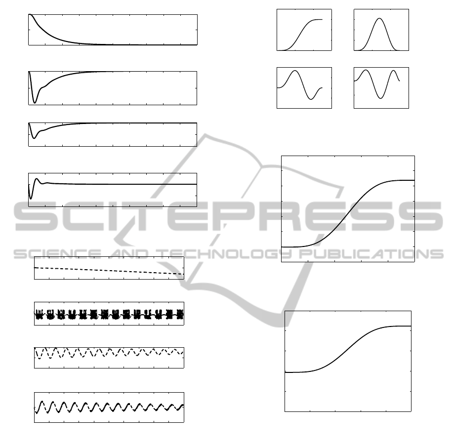
loop behavior of the flexible joint robot without any
control can be seen in figures 5 and 6. Figure 5 indi-
cates the motor position dropping from a position of
1rads under gravity and no voltage applied to the mo-
tors. The motor completely drops the flexible link to
a zero position under gravity in about 2seconds. The
link deflection shows a deflection of about −0.12rads
before returning to zero.
FlatnessbasedFeed-forwardControlofaFlexibleRobotArmunderGravityandJointFriction
177
0 0.5 1 1.5 2 2.5 3 3.5 4 4.5 5
0
0.5
1
Time [s]
Radians
θ
0 0.5 1 1.5 2 2.5 3 3.5 4 4.5 5
−2
−1
0
Time [s]
Rads/s
˙
θ
0 0.5 1 1.5 2 2.5 3 3.5 4 4.5 5
−0.2
−0.1
0
Time [s]
Radians
α
0 0.5 1 1.5 2 2.5 3 3.5 4 4.5 5
−2
−1
0
1
Time [s]
Rads/s
˙α
Figure 5: Open loop robot states under no friction.
0 0.5 1 1.5 2 2.5 3 3.5 4 4.5 5
0.5
1
1.5
Time [s]
Radians
θ
0 0.5 1 1.5 2 2.5 3 3.5 4 4.5 5
−0.5
0
0.5
Time [s]
Rads/s
˙
θ
0 0.5 1 1.5 2 2.5 3 3.5 4 4.5 5
−0.4
−0.2
0
Time [s]
Radians
α
0 0.5 1 1.5 2 2.5 3 3.5 4 4.5 5
−5
0
5
Time [s]
Rads/s
˙α
Figure 6: open loop robot states under friction.
With friction at the joint, figure 6 shows that the
friction slows down the movement of the link towards
the zero position. Within the 5minutes simulation
time, the motor position was still at above the 0.5rads
mark. It takes a longer time to dampen to zero. The
link deflection α shows a lot of oscillations and the
velocities also show strong oscillatory behavior. This
kind of scenarios are undesirable and are a motivation
for designing the flatness based feedforward control
to overcome these nonlinear effects.
Using the flat output equation 17, rest to rest tra-
jectories are generated for the flexible robot arm as
shown in figure 7. These trajectories are now used
to define the feedforward control while compensating
0 2 4 6
0
0.02
0.04
0.06
0.08
y(rads)
time (s)
0 2 4 6
0
0.005
0.01
0.015
0.02
vel(rads/s)
time (s)
0 2 4 6
−0.02
−0.01
0
0.01
0.02
acc(rads/s
2
)
time (s)
0 2 4 6
−0.04
−0.02
0
0.02
jerk(rads/s
3
)
time (s)
Figure 7: Rest to rest trajectories for the flexible joint robot.
0 1 2 3 4 5
3.22
3.23
3.24
3.25
3.26
3.27
3.28
3.29
Torque (NM)
time (s)
Torque
Figure 8: Open loop torque.
0 1 2 3 4 5
8.3
8.35
8.4
8.45
8.5
8.55
u (V)
time (s)
control effort
Figure 9: Open loop voltage.
for the undesirable nonlinear effects that were seen
in the open loop behavior of figures 5 and 6. The
torque and control voltage generated by the flat out-
put to drive the flexible robot arm under gravity and
friction from a zero position to a position of 0.06rads
without any oscillations are shown in figures 8 and
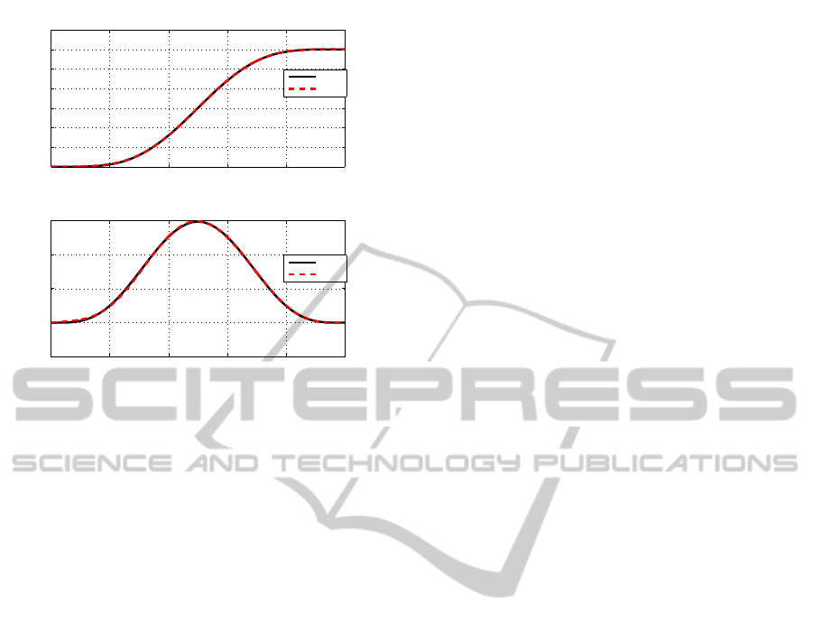
9 respectively. The proposed flatness based feedfor-
ward control designed in equation 10 is then applied
to drive the robot from a position of 0 to 0.06rads. The
result in figure 10 shows that the robot is easily driven
along this path without having to integrate any equa-
tions. The robot arm is able to follow its reference po-
sition without errors. It is assumed that disturbances
are non existent or are kept at a minimum.
ICINCO2015-12thInternationalConferenceonInformaticsinControl,AutomationandRobotics
178
0 0.2 0.4 0.6 0.8 1
0
0.01
0.02
0.03
0.04
0.05
0.06
0.07
Time [s]
Radians
y
ref
actual
0 0.2 0.4 0.6 0.8 1
−0.05
0
0.05
0.1
0.15
Time [s]
Rads/s
˙y
ref
actual
Figure 10: Trajectories driven by flatness based feedfor-
ward control.
6 CONCLUSION
The feedforward control for the single link flexible
joint robot arm under the influence of gravity and fric-
tional effects is solved using differential flatness the-
ory. The control was accomplished for point to point
position movements in finite time. The technique
does not require any solution of differential equations
despite the highly nonlinear dynamics of the robot.
The proposed control has great potential for carrying
out fast and precise point to point movements with-
out any oscillations for the flexible robot arm. The
proposed approach can be extended to the case of
multi-link robot control where elasticity is considered
at each joint and the effects of gravity taken into ac-
count. This will be studied in future works.
REFERENCES
Anene, E. (2007). Flat control of a synchronous machine.
Unpublished Thesis.
Bauer, D., Schaper, U., Schneider, K., and Sawodny, O.
(2014). Observer design and flatness-based feedfor-
ward control with model predictive trajectory plan-
ning of a crane rotator. In American Control Confer-
ence (ACC), 2014, pages 4020–4025. IEEE.
Cambera, J. C., Chocoteco, J. A., and Feliu, V.
(2014). Feedback linearizing controller for a flexi-
ble single-link arm under gravity and joint friction.
In ROBOT2013 First Iberian Robotics Conference,
pages 169–184. Springer.
De Vries, E., Fehn, A., and Rixen, D. (2010). Flatness-
based model inverse for feed-forward braking control.
Vehicle System Dynamics, 48(S1):353–372.
Dwivedy, S. and Eberhard, P. (2006). Dynamic analysis of
flexible manipulators, a literature review. Mechanism
and Machine Theory, 41(7):749–777.
Fliess, M., Levine, J., Martin, P., Ollivier, F., and Rouchon,
P. (1997). Controlling nonlinear systems by flatness.
Systems and Control in the Twenty-first Century, page
137154.
Fliess, M., Levine, J., Martin, P., and Rouchon, P. (1999). A
lie-backlund approach to equivalence and flatness of
nonlinear systems. Automatic Control, IEEE Transac-
tions on, 44(5):922–937.
Hagenmeyer, V. and Delaleau, E. (2003). Exact feedfor-
ward linearization based on differential flatness. In-
ternational Journal of Control, 76(6):537–556.
Ider, S. and zgren, M. (2000). Trajectory tracking control
of flexible-joint robots. Computers and Structures,
76(6):757–763.
Jiang, Z. and Higaki, S. (2011). Control of flexible joint
robot manipulators using a combined controller with
neural network and linear regulator. Proceedings of
the Institution of Mechanical Engineers, Part I: Jour-
nal of Systems and Control Engineering, 225(6):798–
806.
Kandroodi, M., Mansouri, M., Shoorehdeli, M., and Tesh-
nehlab, M. (2012). Control of flexible joint manipu-
lator via reduced rule-based fuzzy control with exper-
imental validation. International Scholarly Research
Network ISRN Artificial Intelligence.
Kharitonov, A. and Sawodny, O. (2006). Flatness-based
feedforward control for parabolic distributed param-
eter systems with distributed control. International
Journal of Control, 79(07):677–687.
Kotman, P., Bitzer, M., and Kugi, A. (2010). Flatness-based
feedforward control of a two-stage turbocharged
diesel air system with egr. In Control Applica-
tions (CCA), 2010 IEEE International Conference on,
pages 979–984. IEEE.
Levine, J. (2006). On necessary and sufficient conditions
for differential flatness. Arxiv preprint math/0605405.
Levine, J. (2009). Analysis and control of nonlinear sys-
tems: A flatness-based approach. Springer.
Markus, E., Agee, J., and Jimoh, A. (2013). Differentially
flat trajectory control of a 6dof industrial robot manip-
ulator. In International Association for Science and
Technology (IASTED)Control and Application confer-
ence, pages 215–221. Iasted.
Markus, E., Agee, J., Jimoh, A., and Tlale, N. (2012a).
Nonlinear control of a single-link flexible joint ma-
nipulator using differential flatness. In Robotics and
Mechatronics Conference (ROBMECH). IEEE.
Markus, E., Agee, J., Jimoh, A., Tlale, N., and Zafer, B.
(2012b). Flatness based control of a 2 dof single
link flexible joint manipulator. In 2nd International
Conferenceon Simulation and Modeling Methodolo-
gies, Technologies and Applications, pages 437–442.
SciTePress.
FlatnessbasedFeed-forwardControlofaFlexibleRobotArmunderGravityandJointFriction
179

Morandini, M., Masarati, P., Bargigli, L., and Vaccani, L.
(2012). Feedforward control design from general-
purpose multibody analysis for an original parallel
robot concept. In Proceedings of the 2nd Joint Inter-
national Conference on Multibody System Dynamics,
P. Eberhard and P. Ziegler, eds., Stuttgart, Germany.
Muller, B., Deutscher, J., and Grodde, S. (2006). Trajec-
tory generation and feedforward control for parking a
car. In Computer Aided Control System Design, 2006
IEEE International Conference on Control Applica-
tions, 2006 IEEE International Symposium on Intelli-
gent Control, 2006 IEEE, pages 163–168. IEEE.
Ozgoli, S. and Taghirad, H. (2006). A survey on the con-
trol of flexible joint robots. Asian Journal of Control,
8(4):332–344.
Palli, G., Borghesan, G., and Melchiorri, C. (2009).
Tendon-based transmission systems for robotic de-
vices: Models and control algorithms. In Robotics
and Automation, 2009. ICRA’09. IEEE International
Conference on, pages 4063–4068. IEEE.
Pereira, E., Becedas, J., Payo, I., Ramos, F., and Feliu, V.
(2007). Control of flexible manipulators. theory and
practice.
Quanser (2015).
Reyes, F. and Kelly, R. (2001). Experimental evaluation of
model-based controllers on a direct-drive robot arm.
Mechatronics, 11(3):267–282.
Rodriguez, A. S.-M., Ibanez, J. C. C., and Battle, V. F.
(2014). Online algebraic identification of the payload
changes in a single-link flexible manipulator moving
under gravity.
Rouchon, P., Fliess, M., Levine, J., and Martin, P. (1993).
Flatness, motion planning and trailer systems. pages
2700–2705 vol. 3. IEEE.
Schlipf, D. and Cheng, P. W. Flatness-based feedforward
control of wind turbines using. In Proceedings of the
19th World Congress of the. Universit¨at Stuttgart.
Tokhi, M. and Azad, A. (2008). Flexible robot manipula-
tors: modelling, simulation and control. In IET Con-
trol Series, volume 68. London Institution of Engi-
neering and Technology.
APPENDIX
The equations for A and B are given here in the ap-
pendix due to their size:
A =
1 1 ... 1
n+ 1 n+ 2 ... 2n+ 1
n.n+ 1 n + 1.n+ 2 ... 2n.2n + 1
n− 1.n.n+ 1 n.n+ 1.n+ 2 ... 2n− 1.2n.2n + 1
. . ... .
. . ... .
. . ... .
(n+ 1)!
(n+2)!
2!
...
(2n+1)!
(n+1)!
−1
and
B =
y(t
2
) − y(t
1
) −
∑
j
1
i!
y
i
(t
1
)(t
2
− t
1
)
i
; fori = 1− n
y
(i−1)
(t
2
) − y
(i−1)
(t
1
)(t
2
− t
1
)
i−1
−
∑
j
1
(i−1)!
y
i
(t
1
)(t
2
− t
1
)
i
; fori = 2− n
y
(i−1)
(t
2
) − y
(i−1)
(t
1
)(t
2
− t
1
)
i−1
−
∑
j
1
(i−2)!
y
i
(t
1
)(t
2
− t
1
)
i
; fori = 3− n
.
.
.
y
i
(t
2
) − y
i
(t
1
)(t
2
− t
1
)
i
; fori = n
ICINCO2015-12thInternationalConferenceonInformaticsinControl,AutomationandRobotics
180
