Statistical Model Checking of GSPN Models

Franco Cicirelli, Christian Nigro and Libero Nigro

Laboratorio di Ingegneria del Software, Dipartimento di Ingegneria Informatica Modellistica Elettronica e Sistemistica

(DIMES), Università della Calabria, Rende, Italy

Keywords: Statistical Model Checking, UPPAAL, Generalized Stochastic Petri Nets, Structural Translation, Temporal

Analysis.

Abstract: Generalized Stochastic Petri Nets (GSPN) are a well-known timed extension of Petri nets suited for

modelling and performance analysis of general time-dependent concurrent systems. The work described in

this paper develops an original structural translation of GSPN models onto U

PPAAL SMC so as to enable

property estimation through statistical model checking. The actual GSPN supported formal language admits,

in general, tagged tokens carrying timestamps, queuing places, normal, transport and inhibitor arcs and

timed and untimed transitions. This paper describes the proposed approach and demonstrates its practical

usefulness through a case study.

1 INTRODUCTION

Generalized Stochastic Petri Nets (GSPN) (Chiola et

al., 1993)(Marsan et al., 2004) are a well-known

timed extension of Petri nets suited for modelling

and performance analysis of general time-dependent

concurrent and distributed systems. Property

checking of GSPN models can be formally based on

the generation of the underlying Continuous Time

Markov Chain (CTMC) state reachability graph

(Marsan et al., 2004) or, in the practical cases of

complex systems whose state graph can suffer of

state explosion problems, through discrete-event

simulation.

In the work described in this paper the GSPN

formalism is mapped on top of the statistical model

checker of the U

PPAAL toolbox (David et al., 2015)

which operates on a network of timed automata

(TA). U

PPAAL was chosen because it is popular,

efficient and enriches TA with data

variables/structures, functions, clocks and

communication channels. U

PPAAL makes it possible

to check system properties using either or both

symbolic model checking (i.e., exhaustive

verification of system behavior on the model state

graph) or statistical model checking (SMC) (Younes,

2005).

SMC does not build the state graph but instead

depends on a batch of simulation runs, possibly

executed in parallel on a modern multicore machine,

and on statistics techniques applied to the results of

these runs. SMC works on a stochastic

interpretations of TA (STA) and can furnish an

estimation of system behavior when the symbolic

state graph of the TA network is prohibitive to be

built in memory or it is undecidable. SMC, instead,

does not suffer of memory problems and can be used

with scalable models.

An original structural translation as in (Cicirelli

et al, 2012) is proposed in this paper which

transforms a GSPN model onto a network of

stochastic timed automata. The actual supported

GSPN formalism can work with classic

indistinguishable tokens or with tagged tokens so as

to allow specifying customer-centric performance

queries. Tagged tokens carry timestamps and are

stored into queue managed places. Arcs can be

normal, transport (Jacobsen et al., 2011) or inhibitor

arcs. Transitions can be timed or untimed (i.e.,

immediate).

With respect to classic special-case GSPN

simulators, the use of U

PPAAL SMC is interesting

because it enables model-specific performance

queries and easily permits to explore design

alternatives. In addition, the built-in visualization

support proves of great value for the modeler.

The rest of this paper is structured as follows.

Section 2 summarizes the basic definitions and

informal semantics of GSPN and illustrates the

modelling capabilities through an example. Section

Cicirelli F., Nigro C. and Nigro L..

Statistical Model Checking of GSPN Models.

DOI: 10.5220/0005506700690076

In Proceedings of the 5th International Conference on Simulation and Modeling Methodologies, Technologies and Applications (SIMULTECH-2015),

pages 69-76

ISBN: 978-989-758-120-5

 2015 SCITEPRESS (Science and Technology Publications, Lda.)

3 describes the proposed structural translation of

GSPN onto UPPAAL SMC. Section 4 shows the

statistical model checking of the GSPN model

proposed in Section 2. Finally, conclusions are

presented with an indication of research directions

which deserve further work.

2 GSPN CONCEPTS

2.1 Basic Definitions

A basic GSPN is a tuple , 



,



,,,



,



,,

,  where:

  is a finite nonempty set of places;

 



∪



is a finite nonempty set of

transitions, where 



 is the subset of timed

transitions, 



⊂ is the set of immediate (or

untimed) transitions;

 ∩∅;

 Bis the backward incidence function, :  

→, where  denotes the set of natural

numbers;

  is the forward incidence function, :   →

;

 



is the set of inhibitor arcs, 



⊂

where



, 



∈



⇒



, 



0;

 



is the initial marking function, 



: → ,

which associates with each place a number of

tokens;

 : 



→



is a function which associates each

timed transition with a firing delay, i.e., the rate

of an exponential probability distribution

function. 



denotes the set of positive real

numbers;

 : 



→0,1 is a function that associates each

immediate transition with a probability value;

 : 



→ is a function which associates each

immediate transition with a priority value.

2.2 Informal Semantics

Let :  →  be the marking function of a GSPN.

As in classic Petri nets, a transition ∈ is said to

be enabled in  iff ∀ ∈ ,



, 



∈



⇒









0 ∧ 



, 



0⇒











, 



. An enabled

transition  is fireable. Firing of  changes

(instantaneously and atomically) the current marking

 into a new marking 



such that: ∀ ∈ ,























, 







, 



If both immediate and timed transitions are

enabled in , the firing of immediate transitions

precedes the firing of timed transitions. Among the

immediate transitions, first priorities are applied. To

choice among immediate transitions having the same

highest priority, probabilities are applied. When

there are no more enabled immediate transitions,

timed transitions are allowed to fire according to

their absolute fire time established at the enabling

time by adding a sample (relative firing delay)

achieved from the associated exponential

distribution, to the current time. The most imminent

firing time dictates the timed transition to fire.

In this work the following policies regulate the

firing of timed transitions: (a) single-server

semantics, i.e., each transition fires its enablings one

at a time and sequentially, (b) race with re-sampling,

that is non determinism is applied when multiple

transitions should fire at the same time, and the

remaining time to fire is not memorized at a

transition preemption caused by the firing of a

conflicting transition. As a consequence of the

single-server semantics, a multi-server behavior

(parallel server), when needed, has to be explicitly

obtained in the model by replicating the server timed

transition (see transitions from

t0 to t9 in the upper

section of the model in Fig. 2). The atomic and

instantaneous firing process of any transition is

actually split into the two phases: withdrawl and

deposit of tokens. A transition  can loss its enabling

just after the withdrawl phase or the deposit phase of

the firing of another transition 



. Whichever the

case, transition  which loses its enabling is

immediately preempted.

2.2.1 Modelling Extensions

For the purposes of this paper, GSPN modelling is

extended by admitting also timed transitions with a

uniform distribution. In addition, to simplify the

performance analysis of some models, tokens can be

tagged, thus enabling a client-specific expression of

performance queries. Tagging means a token is

attached a unique identifier which in turn associates

the token with a timer (timestamp or age) carrying

the elapsed time since its last reset.

Besides normal arcs, the notion of a transport

arc (Jacobsen et al., 2011) is added to allow a token

to move from a place to another, during a transition

firing, while retaining its updated age. To clarify the

couple of places involved in a transport operation,

the notation “:arc-label”, with arc-label a natural

number, is attached to the couple of transport arcs

(see Fig. 1).

When a token is generated through a normal

output arc, its timer is reset. A dynamic tagging

system is actually adopted, supported by a pool of

available tags. Since classic transition firing involves

SIMULTECH2015-5thInternationalConferenceonSimulationandModelingMethodologies,Technologiesand

Applications

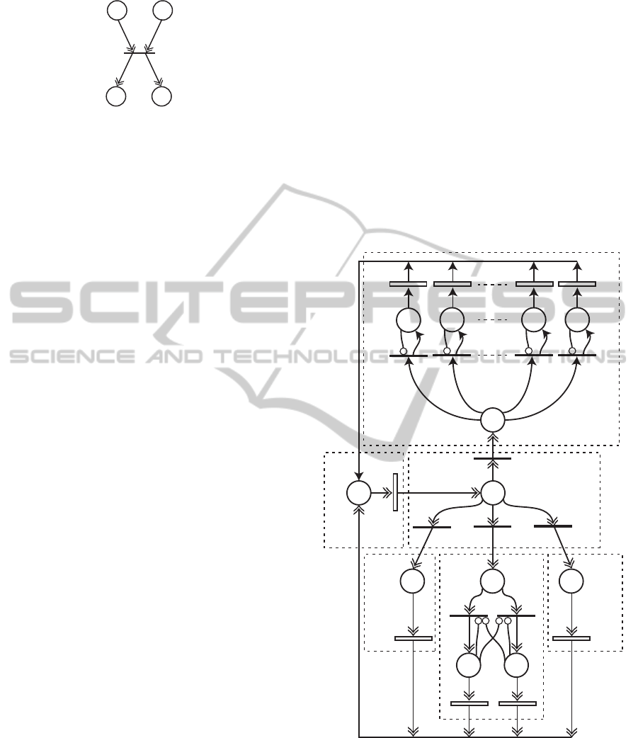
Figure 1: Two couples of transport arcs.

only normal arcs and operates on anonym tokens, it

is possible to release to the pool the tags of

withdrawn tokens and acquire tags from the pool

(and reset their timers) for newly generated tokens.

The association of tags to tokens has to be kept, with

the help of transport arcs, when it is important to

observe the elapsed time from a cause event to an

effect event. The use of tagged tokens is

complemented with a notion of queue managed

places. Whereas anonym tokens imply a random

policy can be used to select tokens during a

withdrawl phase, in a queue managed place, instead,

tokens are stored and retrieved according to their

arrival time. Finally, to simplify model expression

the following defaults and conventions are adopted

(see also Fig. 2). Timed transitions are depicted as

small white rectangles, whereas immediate

transitions as black thin bars. Transport arcs are

drawn as double ended arrows, normal arcs as single

ended arrows, inhibitor arcs are terminated by a

small circle. Ordinary arcs, i.e., having a unitary

weight, can be introduced without weight

specification. Similarly, when there is no need to

distinguish among the transport arcs, the

specification is implicitly assumed. When not

explicitly indicated, the default priority value

=1

applies to immediate transitions.

2.3 A Modelling Example

Fig. 2 portrays a GSPN model where a fixed number

of clients recirculate and attend for service in the

system. The model is the interconnection of six

components (stations or service centers). S0 is a

reflective station. Here clients reflect in parallel

before entering the system, i.e. moving in input to

the S1 station. After being served by S1, a client can

be redirected to one of three specific service centers

S2, S3 or S4, or it can exit the system by re-entering

the S0 station. The choice is performed by a Router

station which realizes a random switch. After being

served by S2, S3 or S4, a client comes back in input

to S1, ready for a new cycle in the system.

The model is representative of many physical

systems. For instance, it can describe the operation

of a call center (Cicirelli and Nigro, 2015), or the

accident and emergency unit of an hospital etc. The

parameter values in Fig. 2 are just an example to

drive a case study. A population of

10 clients is

considered. S1 and S2 are simple exponential

distributed stations.

S4 follows an Erlang

distribution composed of 16 exponential

distributions all having the same rate =0.6. The

Erlang distribution was abstracted as one

exponential distribution of rate

14=0.6/16=0.0375.

S3 adopts an hyper-exponential distribution made up

of two exponential distributions able to generate a

burst behavior. Here, for demonstration purposes, a

subnet is used to further exemplify the use of

probabilities for controlling a random switch.

Router

S2 S3

P15

P16

P2 P9 P10

=0.1

=0.1 λ

=0.1

=0.8 λ

=0.0375

= 5.0 λ

= 0.5

=0.3

=0.2

0.95

0.05

P13

P14 P17

P12P11

=0.2

Figure 2: A GSPN model for a system of services.

As one can see from Fig. 2, the model is logically

split in two sections. The upper section hosts the

reflective station and makes use of normal arcs only.

When a client finishes reflecting (a transition

between

t0 to t9 fires), it is injected into the p11

place and its timer is reset. The lower section

StatisticalModelCheckingofGSPNModels

contains the effective service system. Here transport

arcs are used to allow tracking the temporal behavior

of each client as it flows from one station to another.

When a client is routed to

p0 it exits the system and

enters the reflective station. At each firing of t25, the

token timestamp mirrors the sojourn time of the

client in the system. The model will be analyzed

later in this paper, by evaluating the throughput,

utilization, response time etc. separately for each

station and as emerging properties of the whole

system. In addition, some specific properties such as

estimating the probability a certain number of clients

consecutively exits the system with each client

having experimented a sojourn time less than or

equal to a given end-to-end delay (deadline), will be

investigated.

3 A STRUCTURAL

TRANSLATION OF GSPN

ONTO UPPAAL

GSPN models can be transformed into UPPAAL

SMC (David et al, 2015) by associating each

transition with a suitable template process and by

introducing some global data and helper functions.

The following constants capture model topology:

P (number of places), PRE (maximum number of

input places per transition),

POST (maximum

number of output places per transition),

T (number

of transitions),

ET (number of exponential

transitions),

UT (number of uniform transitions), IT

(number of immediate transitions), T=ET+UT+IT, B

and F (incidence matrices), M (marking vector),

TAGS (number of available tags), MTA (maximum

number of distinct transport arcs). The three

constants

NORMAL, TRANSPORT and INHIBITOR

denote the corresponding arc type. Each element of

the matrices

B and F, implemented as TxPRE and

TxPOST respectively, holds the index of a place, the

weight of an arc, the type of the arc and the id of the

transport arc if the previous attribute is

TRANSPORT.

Transitions are numbered from

0 to T-1. In

particular (see also Fig. 2), as a matter of

convention, first are numbered the exponential

transitions, then the uniform transitions, finally the

immediate transitions.

tid is the integer range type of

all transitions, etid, utid and itid are respectively the

range types of the three categories of transitions. pid

is the range type of places. tags is the range type of

the tags,

atid and taid respectively describe the range

type of arcs and of the transport arcs. Global

functions

bool enabled(tid), void withdraw(tid), void

deposit(tid) respectively check transition enabling

and realize token withdrawal and deposit during a

transition firing. Global function

void rank() returns

in the global variable NIT the id of the Next

Immediate Transition to fire. The clock array

y[ET+UT] associates a clock to each timed transition.

The clocks in y serve the purpose of measuring

transitions activity periods. They are stopped when

the transition is disabled. The clock array

x[UT]

associates a clock with every uniform transition.

Each clock in

x is used to constrain the firing of the

transition according to its time interval. The global

clock

now mirrors current system time. Clock stime

is devoted to measuring the activity periods of the

system. The clock array

time[TAGS] associates a

clock to each distinct tag. The global array ta[MTA]

stores the tags flowing through specific transport

arcs during a transition firing. The global array

pool[TAGS] along with the top variable realize a

stack of dynamically available tags. The tag pool is

actually managed by the functions

tags acquire() and

void release(tags). The global queue structure

implements the tag queue associated with each

place. The array

queue tag[pid] associates each place

with its tag queue. Tag queues are managed by the

functions:

void enq(&queue,tags), tags deq(&queue),

bool empty (queue), bool full(queue), tags

size(queue).

3.1 Template Models

Figures from 3 to 5 depict the three basic automata

corresponding to timed (exponential or uniform) and

untimed (immediate) transitions of a GSPN model.

Figure 3: The eTransition automaton.

Basic design issues can be described through the

eTransition automaton (Fig. 3). An eTransition t

borns in the

N (Not enabled) location. It moves to

the F (Fireable) location as soon as it finds itself

enabled. In F the transition can remain a time

corresponding to a sample of the exponential

probability distribution whose rate (possibly

marking dependent) is furnished by the function

!enabled(t)

enabled(t)

NIT==NONE

enabled(t)

end_fire!

end_fire!!enabled(t)

end_fire?

end_fire! deposit(t)

fire=false

rate(t)

withdraw(t),

fire=true

fire=false

y[t]'==0

SIMULTECH2015-5thInternationalConferenceonSimulationandModelingMethodologies,Technologiesand

Applications

rate(t). The transition can complete its firing

provided no immediate transition is under firing

(

NIT==NONE). If the transition loses its enabling

during its stay in F, it immediately comes back to N.

The firing process of t is completed by performing

(atomically and instantaneously) the two sub-phases

of withdraw and deposit of tokens. Towards this the

broadcast

end_fire channel is used together with the

two committed locations

W and D. Two end_fire

synchronizations are actually launched by transition

t respectively after the withdraw and the deposit

phases. Each synchronization forces all the other

transitions to review their enabling status following

the firing of

t. Movements from N to F or from F to

N are triggered by receiving an end_fire?

synchronization (another transition is completing its

firing) and the check of the enabling status. It is

worth noting that all the three templates make it

possible to enable/disable other transitions at the end

of each sub-phase of a firing. An

eTransition t stops

its clock

y[t] when it stays in N. The clock is

reactivated as soon as the transition abandons N.

Figure 4: The uTransition automaton.

An uTransition automaton t behaves in a similar way

to an eTransition. The difference is that now there is

an interval [lb(t),ub(t)] for the firing time, with

lb(t)<=ub(t) and ub(t) can be infinite (expressed by

the global constant INF). Global functions lb(t), ub(t)

return respectively the lower and upper bounds

(possibly marking dependent) of

t. The upper section

of the uTransition automaton is related to a time

strict interval, i.e.,

ub(t)!=INF. The lower section

handles the cases of [lb(t),INF]. Let us first consider a

time strict interval. As soon as t discovers it is

enabled, it moves to the

F location and resets its

clock x[t]. Transition firing is then constrained to

occur at an instant within

[lb(t),ub[t]. The invariant

x[t]<=ub(t) attached to F forces the exiting from F

would the last instant of the interval have been

reached, provided the transition is still enabled and

no fireable immediate transition exists at the

moment. The firing edge leaving

F is conditioned by

the guard

x[t]>=lb(t) to ensure the transition cannot

fire before the lower bound is not yet elapsed. The

lower section in Fig. 4 first guarantees the lower

bound is elapsed (location

F1). Then the automaton

moves to the F2 location where it waits for an

amount of time established by a model provided

exponential distribution whose rate is given by

rate(t).

Figure 5: The iTransition automaton.

An iTransition automaton t behaves as shown in Fig.

5. A major difference from Fig. 3 and 4 is the

location

F is now committed, i.e., the transition has

to fire immediately. All the enabled immediate

transitions in the current marking reach

simultaneously their

F location. It is the

responsibility of the

rank() function that of selecting

the id of the next immediate transition to fire (held

in the global variable

NIT), by first applying

priorities and then probabilities (the U

PPAAL SMC

library function

random(b) is exploited). To avoid

interleaving of committed locations, an immediate

transition is allowed to fire only if there is a not in

progress firing of a timed transition (see the global

fire variable).

Figure 6: The SystemMonitor automaton.

For model bootstrapping a Starter automaton is used

which invokes a

model_initialize() function (model

specific) and then launches a first

end_fire

enabled(t)&&

ub(t)==INF

x[t]>=lb(t)

enabled(t)&&

ub(t)!=INF

!enabled(t)

enabled(t)&&

ub(t)==INF

NIT==NONE

!enabled(t)

end_fire!

end_fire?

x[t]>=lb(t) &&

NIT==NONE

end_fire!

enabled(t)&&

ub(t)!=INF

end_fire?

withdraw(t),

fire=true

deposit(t)

x[t]=0

rate(t)

x[t]<=lb(t)

withdraw(t),

fire=true

x[t]=0,fire=false

fire=false

x[t]=0

x[t]=0,fire=false

x[t]<=ub(t)

y[t]'==0

!enabled(t)

enabled(t)enabled(t)

end_fire!

!fire && t==NIT

end_fire?

!enabled(t)

end_fire!

withdraw(t),

NIT=NONE

deposit(t)rank()

rank()rank()

idle active

activate()

end_fire?

stime'==0

deactivate()

StatisticalModelCheckingofGSPNModels

synchronization. In Fig. 6 it is portrayed an

automaton which monitors system activity and

permits to collect information about the entire

system. For the model in Fig. 2,

activate() returns

true if at least one token is found within the places

p11, p13, p15, p16 and p17, and conversely for

deactivate().

4 SMC ANALYSIS OF GSPN

MODEL

The following reports some experimental results

about the GSPN model in Fig. 2 preliminarily

translated in U

PPAAL SMC.

In order to get statistical information about the

temporal behavior of the GSPN model, a problem-

specific decoration was added to the translated

model. Some global arrays were introduced to

observe the number of services (

n[]), the utilization

(u[]), the throughput (thru[]), the response time (rt[])

and mean service time (st[]) of each station. Simple

variables sn, su, sthru, srt allow to watch emergent

properties of the whole system. It is worth noting

that all the reported pictures were directly taken

from U

PPAAL SMC.

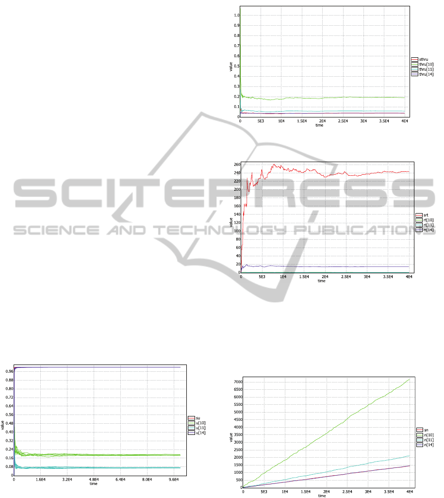
The attainment of steady-state condition (see Fig.

7) was checked by monitoring the utilization of the

system and of the selected transitions

t10 (S1), t11

(S2) and t14 (S4) of Fig. 2, using 5 simulations with

as the time limit, by the query:

simulate 5 [<=100000] { su, u[10], u[11], u[14] }

Figure 7: Utilization of system and of S1, S2 and S4.

As one can see from Fig. 7, 3x10

tu are sufficient to

reach the steady-state.

One goal of the performance study was to detect

sources of bottlenecks, if any, for the system

behavior. From Fig. 7 it results that system

utilization and

S4 utilization are both 100%, whereas

the utilization of other stations is lower, in particular

the

S2 utilization is the lowest one.

Figure 8: Throughput of system and of S1, S2 and S4.

Figure 9: Response time of the system and of S1, S2 and

S4.

Fig. 8 and 9 show the throughput (number of served

clients per time unit) and response time (i.e., client

waiting time for service plus service time) for the

same components (using 1 simulation of

4x10

tu).

Figure 10: Number of services vs. time.

The system exhibits the same throughput of S4,

suggesting S4 could be a performance bottleneck for

the system. The response time of S4 is greater than

that of

S1. The intuition that S4 is effectively a

bottleneck for system behavior is confirmed also by

Fig. 10 where the number of performed services is

SIMULTECH2015-5thInternationalConferenceonSimulationandModelingMethodologies,Technologiesand

Applications

shown. Here the number of services realized by the

system coincides with that of S4.

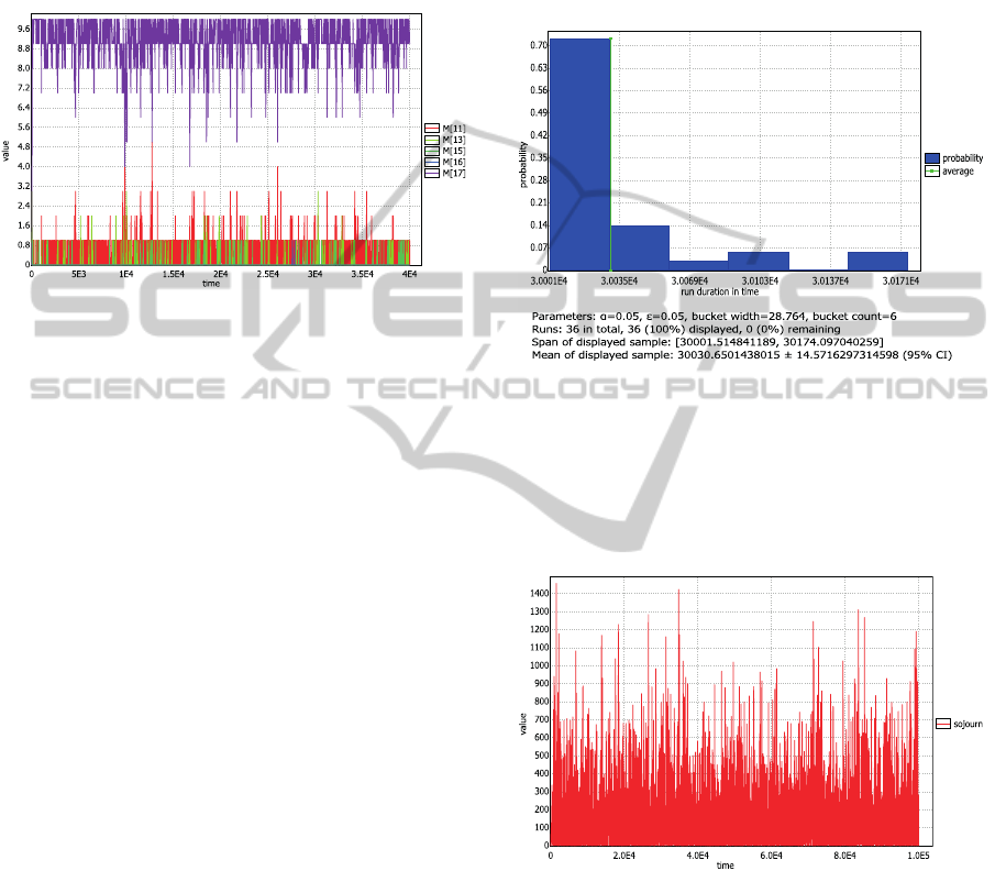
Fig. 11 portrays the marking (queue length) of

the various stations, which was monitored using the

query:

simulate 1 [<=40000] { M[11],M[13],M[15],M[16],M[17] }

Figure 11: Station queue lengths vs. time.

As it clearly emerges from the Fig. 11, most of the

time clients get sticked into the place p17, as the

marking of

M[17] is almost often close to 10 (recall

the system model admits 10 recirculating clients).

The resultant behavior confirmed the modeler

expectation being

S14 the station with the highest

mean service time (1/0.0375=26.667 tu).

The performance pictures were re-generated with

the service rate of station S4 being doubled

(

14=0.0750). As the mean service time of S4

remains the highest one among the various stations,

it still drives the emergent system behavior, although

now the distribution of clients among the stations

was found improved and the number of services

doubled.

Estimating the response times depicted in Fig. 9

was facilitated by token tagging.

As a specific property based on client-tracking

(assuming

14=0.0750), it was checked the event E1

“What is the probability of a client exiting the system

with a sojourn time not greater than the deadline

D=50 tu?”. The following query was issued:

Pr[<=100000] (<>now>=30000 &&

iTransition(25).W && time[ta[0]]<=D )

The query eliminates transient behavior by ensuring

the

now clock is greater than 30000 tu. Then, the

firing of the immediate transition iTransition(25)

(i.e., t25 in Fig. 2) is considered along with the client

time checked against the deadline. It should be noted

that when

iTransition(25) fires (that is the withdraw

W location is entered in Fig. 5), the tag (identifier) of

the token (client) can be retrieved as ta[0], which is

then used to select the client clock (time[ta[0]]) to

compare against the chosen deadline. Fig. 12 depicts

a probability distribution of the event whose

confidence interval (CI) is

[0.902606,1] with a 95%

confidence degree (CD). UPPAAL SMC used 36 runs

to estimate the query result and the plot refers to a

time sample chosen by the tool in which the runs

satisfy the query.

Figure 12: A probability distribution for the eventE1.

Whereas the response times reported in Fig. 9 are

average values, Fig. 13 plots measured values of the

system sojourn time of clients during a simulation

experiment. It emerges a maximum value of about

1400 tu.

Figure 13: Observed sojourn time during a simulation

The next step was checking the probability of the

event E2 “What is the probability the percentage of

clients which exit the system with a sojourn time less

than or equal to the deadline D=50 tu, be at least

50%?”, using the query:

Pr[<=100000] ( <>now>=30000 && PCSTlteD>=0.50 )

A decoration variable was used to count the number

of clients which exit the system with a sojourn time

less than or equal to the deadline. Such a counter is

divided by the number of services of the system, and

StatisticalModelCheckingofGSPNModels

stored in the percentage variable used in the query.

UPPAAL SMC used 118 runs with a wall clock time

(

WCT) of about 15 min, and suggested a CI for the

event of [0.870781,0.970278] with 95% of CD.

As another property, it was studied the event E3

“What is the probability of 4 consecutive clients

exiting the system with the sojourn time of each

client being not greater than D=50 tu?”.

In this case model decoration was adapted so as

to increment the counter

NCCSTlteD when the

current client exits the system (iTransition(25) fires)

within the deadline and the immediately preceding

one did the same. If current client does not fulfill the

deadline the counter is reset. The following query

was issued:

Pr[<=100000](<>now>=30000 && NCCSTlteD==4)

which generated, with 36 runs, a CI of [0.902606,1]

with 95% CD, and a WCT of 3.5 min.

The following query was used to estimate the

maximum value of the

NCCSTlteD counter using 20

simulation runs.

E[<=100000;20] ( max:NCCSTlteD )

Proposed answer was 13.55±0.93 (WCT of 6.45

min).

Experiments were carried out using a Win 8,

Intel Core i5 CPU @ 2.67 Gz, 8 GB RAM.

5 CONCLUSIONS

In this paper UPPAAL SMC (David et al., 2015) is

exploited for modelling and analysis of Generalized

Stochastic Petri Net (GSPN) models which, besides

working with an arbitrary number of

undistinguishable tokens, can be decorated to work

with tagged tokens.

An original structural translation from GSPN to

stochastic timed automata was developed which

enables a thorough assessment of the temporal

behavior of a modelled system. Practical usefulness

and flexibility of the achieved implementation is

demonstrated by a case study. The example testifies

that a proper decoration of a translated model

enables queries to be designed to check not obvious

system properties. On the other hand, since the state

graph of the model is not generated, added variables

do not constitute a memory penalty for the stochastic

analysis of the model.

Prosecution of the research is geared at:

 Automating the generation of the U

PPAAL SMC

code of a GSPN model using the TPN Designer

toolbox (Carullo et al., 2003).

 Specializing the approach to support modeling

and quantitative evaluation of stochastic Time

Petri Nets (Vicario et al., 2009).

 Experimenting with the use of U

PPAAL SMC in

the modelling and schedulability analysis of

real-time systems.

REFERENCES

Vicario, E., Sassoli, L., Carnevali, L., 2009. Using

Stochastic State Classes in Quantitative Evaluation of

Dense-Time Reactive Systems, IEEE Transactions on

Software Engineering., 35(5):703-719.

Carullo, L., Furfaro, A., Nigro, L., Pupo, F., 2003.

Modelling and Simulation of Complex Systems using

TPN Designer. Simulation Modelling Practice and

Theory. 11/7-8, pp. 503-532.

Chiola, G., Marsan, M. A., Balbo, G., Conte, G., 1993.

Generalized Stochastic Petri Nets: A Definition at the

Net Level and its Implications. IEEE Transactions on

Software Engineering, 19(2):89-107.

Cicirelli, F., Furfaro, A., Nigro, L., 2012. Model Checking Time-

Dependent System Specifications Using Time Stream Petri

Nets and U

PPAAL, Applied Mathematics and Computation,

218(16):8160-8186.

Cicirelli F., Nigro, L., 2015. Control Aspects in Multi-

Agent Systems, Chapter of forthcoming Springer book

Intelligent Agents in Data Intensive Computing, Ed. J.

Kolodziej, L. Correia, and J.M. Molina.

David A., Larsen, K. G., Legay, A., Mikucionis, M.,

Poulsen, D. B., 2015. U

PPAAL SMS Tutorial, Int. J. on

Software Tools for Technology Transfer, Springer,

17:1-19, 06.01.2015, DOI 10.1007/s10009-014-0361-

Jacobsen L., Jacobsen, M., Moller, M. H., Srba, J., 2011.

Verification of Timed-Arc Petri Nets. SOFSEM 2011,

LNCS 6542, pp. 46-72.

Marsan, M. A., Balbo, G., Conte, G., Donatelli, S.,

Franceschinis, G., 2004. Modelling With Generalized

Stochastic Petri Nets. John Wiley and Sons.

Younes, H. L. S., 2005. Verification and Planning for

Stochastic Processes with Asynchronous Events, PhD

Thesis, Carneige Mellon.

SIMULTECH2015-5thInternationalConferenceonSimulationandModelingMethodologies,Technologiesand

Applications