SIM

A Flexible, Scalable and Expandable Simulation Platform Applying to Lunar Orbit

Rendezvous Mission

Sun Fuyu, Wang Hua, Guo Shuai and Li Haiyang

College of Aerospace Science and Engineering, National University of Defense Technology, Changsha, China

Keywords: Distributed Simulation, Layered-design Theory, Model-templet, Simulation Platform, Lunar Orbit

Rendezvous Mission.

Abstract: In this paper we propose a new simulation platform called SIM, for analyzing parallel and distributed

systems. This platform aims to test parallel and distributed architectures and applications. The main

characteristics of SIM are flexibility, scalability and expandability. SIM is about five functions: model

management, experiment management, distribution management, operation management and node

management. To improve the efficiency of project development, new models are designed for lunar orbit

rendezvous mission to apply the simulation platform. Finally, a validation process and evaluation tests have

been performed to evaluate the SIM platform and lunar orbit rendezvous mission models. The simulation

platform and models will lay the foundation for the more validations of autonomy technology in manned

lunar landing research.

1 INTRODUCTION

Nowadays as an important research in aerospace

field manned lunar landing is getting more and more

attention from many space powers such as America,

Russia, and other European countries (Bocam et al.,

2005 and Santovincenzo, 2004). Apollo is the most

representative in the history of exploring the moon.

Lunar orbit rendezvous technology has proved to be

very useful in the Apollo plan (Reeves, 2005).

The methodology of exploring the moon can be

classified into earth orbit rendezvous and lunar orbit

rendezvous. The earth orbit rendezvous method

separates the spacecraft into many modules which

are assembled on the orbit near the earth. As the

mainstream of exploring the moon, the earth orbit

rendezvous method is widely adopted by many

countries such as the Crew Exploration Vehicle of

America (Raftery and Fox, 2007), the Flier plan of

Russia, and the Architecture Study for Sustainable

Lunar Exploration by ESA CDF Study Academy

(Santovincenzo, 2004). The earth orbit rendezvous is

a mature and highly reliable technology, but it needs

more fuel and longer rendezvous period which is

very unbeneficial to the whole mission. The lunar

orbit rendezvous method is to assemble all the

modules of the moon exploring spacecraft on the

lunar orbit. Because of the smaller gravity of the

moon, it costs less fuels to dock on the lunar orbit.

Thence, it is appreciated by more and more countries

as a new method to explore the moon.

Lunar orbit rendezvous is an independent and

complicated mission. It is necessary to verify the

reliability and security of the mission by the

technology of distributed simulation. Many countries

have committed a large number of resources to build

suitable simulation platforms in the related field.

These platforms are playing important roles in the

ground experiment.

Some of these simulators are focused on

simulating. And the entire system provides

functional execution of unmodified commercial

operating systems and applications such as COTSon

(Argollo et al., 2009), a simulator framework jointly

developed by HP Labs and AMD that provides

accurate evaluations of current and future computing;

M5 (Binkert et al., 2006), which supports the

execution of the entire system, including operating

system code, models of network and disk devices;

Simics (Magnusson et al., 2002), another full-system

simulator that was one of the first academic projects

in this area and the first commercial full-system

simulator; and SimOS (Rosenblum et al., 1995 and

Rosenblum et al., 1997), an environment for

Fuyu S., Hua W., Shuai G. and Haiyang L..

SIM - A Flexible, Scalable and Expandable Simulation Platform Applying to Lunar Orbit Rendezvous Mission.

DOI: 10.5220/0005508900770087

In Proceedings of the 5th International Conference on Simulation and Modeling Methodologies, Technologies and Applications (SIMULTECH-2015),

pages 77-87

ISBN: 978-989-758-120-5

 2015 SCITEPRESS (Science and Technology Publications, Lda.)

studying the hardware and software of computer

systems. These simulators are called full-system

simulators. The main advantage of those simulators

is the high level of accuracy obtained, whereas the

main drawback is its performance, which in most

cases is five or six orders of magnitude slower than a

real system.

Moreover, there are approaches that do not focus

on modelling and simulating the system with a full

level of detail instead on balancing the level of detail

to model the system with the performance and

accuracy obtained. For instance, Phantom (Zhai et al.,

2010) proposes a novel approach to predict the

sequential computation time accurately and

efficiently by integrating a computation-time

acquisition approach with a trace-driven network

simulator. dPerf (Cornea and Bourgeois, 2010) is a

tool that uses Rose (Liao et al., 2009) for performing

static analysis of the input source code of programs

written in C, C++, or Fortran.

There are also other works that focused on

distributed storage architectures. One example of

this kind of system is Modeling Infrastructure for

Dynamic Active Storage (MIDAS) (Tarapore et al.,

2008). MIDAS is an execution-driven simulator that

captures both the processing and I/O behavior of

active storage systems. MIDAS simulates a host

system interacting with the I/O path via an

interconnection network. The simulated I/O path can

include disk drives with programmable processors

and programmable storage controllers. The

micro-architecture of each one of these components

is configurable. With this framework, the effects of

different processor micro-architectures, physical disk

and network designs, and communication protocols

on application performance can be explored.

Due to the high number of domains in the field of

distributed systems, developing a universal simulator

is impractical and unfeasible. Naturally, each

researcher has its own objectives and requirements,

and the same way each simulator is developed for a

specific purpose. Many existing simulators do not fit

the researcher’s requirements. As a result,

researchers have to modify an existing simulator, or

coding a new one. But coding a simulator from

scratch is a very complex and difficult task. Usually,

researchers use simulation frameworks for building a

specific simulator.

In this paper, we propose a new simulation

platform called SIM, which is oriented towards

analyzing and studying parallel applications on

distributed systems. SIM has been designed to

provide flexibility, accuracy, performance, and

scalability. Those features make it a powerful

simulation platform for designing, testing and

analyzing both actual and non-existent architectures.

Simulation Systems range from a single computing

node to a complete high performance distributed

system. In fact, this simulation platform has been

applied to data systems simulation in the 921

Manned Space Office of China.

The rest of the paper is structured as follows.

Section 2 presents some requirements. Section 3

describes the basic architecture of SIM. Section 4

shows the strategies and the tools to model

distributed environments in SIM. Section 5 presents

practical implementation and experimental results.

Finally, Section 6 presents some conclusions and

future works.

2 REQUIREMENTS

Actualization of the lunar orbit mission puts forward

higher requirements of the project system such as

higher precision of the lunch vehicle operational

accuracy, more powerful relative navigation or

rendezvous and docking of spacecraft, shorter

response period of measurement and control

communication system, higher precision of

measurement and control instrument. Aspects needed

to be verified from the whole project are:

(1) The Mission Profile Verification

Verifying validity and rationality among the

systems and mission phases of the lunar orbit

rendezvous.

(2) Mission Software Verification

Verifying validity of the software used by the

lunar orbit rendezvous test experiment. These

softwares include lunch window calculation,

orbit determination and fuel injection, spacecraft

GNC.

(3) Flight Control Strategy

Verifying validity of the flight control strategy.

Verifying the effects of orbit error on the flight

control. Verifying the strategy for the orbit

fault-pattern. Verifying the optimal methods of

the flight control.

(4) Visual Presentation for Flight Process

Visual presentation for the whole flight process

of lunar orbit rendezvous. Providing visual image

of 3D scene, subastral point of the flight process.

Considering common problems of simulation

platforms for different kinds of aerospace missions,

we must understand the structure of the new

platform and relationship among function layers

before designing. We must ensure sufficient

versatility, standardization and extendibility of the

SIMULTECH2015-5thInternationalConferenceonSimulationandModelingMethodologies,Technologiesand

Applications

platform. The following points shall be paid

attention to:

(1) Most platforms are suited to only one kind of

models. In the face of complicated aerospace

projects, modeling development is not

complicated by one person or one company. Type

of singleness brings much trouble to the system

integration job.

(2) Most platforms are built for the special missions

in many academies and aerospace institutions.

Simulation platforms are not separated from

models because model program is embedded into

the platform. As models change, the platform

inner structure program will be compiled again.

(3) Most platforms run short of user interface. Only

program structure about initialization, operation,

and reprocessing is exposed by these platforms.

It is not convenient for the experiment design or

visual display.

3 BASIC ARCHITECTURE

Simulation platform is the key of overall simulation

system. In order to meet the integration of different

kinds of models, simulation platform should provide

support for the bottom of different simulation

applications. As it is said that, taking advantage of

universalization, standardization and scalability of

simulation platform, will reduce the difficulty of

system development and the period of model

establishment. Therefore, the quality of a platform is

the evaluation standard for a simulation system. For

a simulation system, its universalization feature

means that the platform is suited to many kinds of

applications. In this paper, they are ground tests to

different kinds of aerospace missions.

Standardization emphasizes specificity among

function-layers, criterion of connections between

platform-platform and platform-model. Scalability is

saying that the SIM simulator is prepared to

cooperate with other simulation tools by performing

different roles. There are two main scenarios:

Integrating an external simulator within SIM or

integrating the SIM framework within another

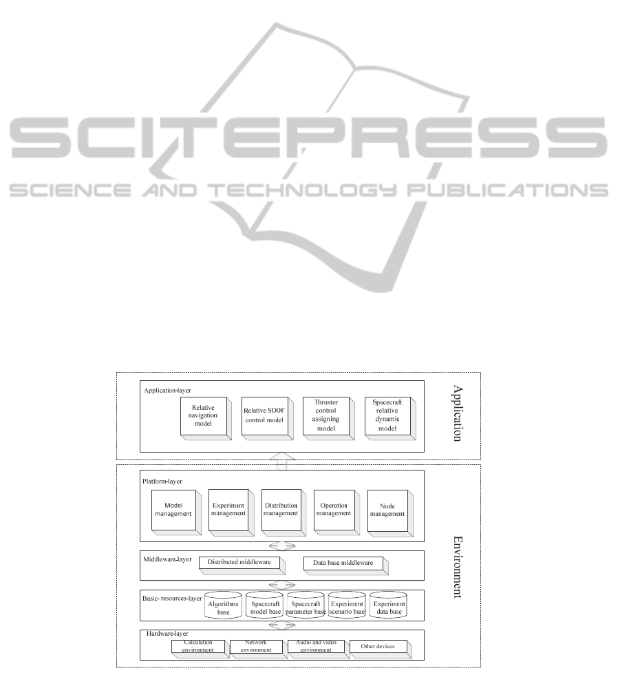
simulator. Figure 1 shows the simulation system

architecture.

SIM simulator consists of model management,

experiment management, distribution management,

operation management and node management.

Model management function can unify different

kinds of models by making operations with the

whole models or amending the information of a

single model. Its design concentrates on

layered-design theory. It realizes the separation

between platform and models, model description and

model realization. It is convenient for modeling,

design of the experiment or the subsequent

construction of simulation system.

Experiment management is mainly to assemble

models with visualization software, configure

connections among models, set model attributes. It

establishes a communication bridge between user

and simulation system. An excellent user interface

does not only bring users enjoyable feelings, but also

Figure 1: The simulation system architecture.

SIM-AFlexible,ScalableandExpandableSimulationPlatformApplyingtoLunarOrbitRendezvousMission

simplify the simulation experiment from foundation

to testament. It is worth mentioning that

layered-design theory is also used in the design

concept of the experiment management. It separates

models and model connections to increase flexibility

of test design and reusability of models.

Distribution management adopts the idea of

“distributed calculation, concentrated management”.

It distributes each model and model parameters to

every node based on simulation scenarios. User can

operate models which are on the node or the

computer itself remotely. Related information will be

shown on the test interface.

Simulation operation management is designed

with responsibility for driving different kinds of

models and attemperring distributedly. Meanwhile, it

can also monitor the state of node and reserve data at

breakpoint.

Node management is disposed on the calculation

node computer with the function of node guard,

model scheduling, and node state reporting. The

function is in cooperation with manager node

computer.

3.1 Model Management

Model management is the most basic and important

function of platform. Each model works as a block.

With the existing of model management function,

simple blocks can be stacked to form the complex

tall building and great mansion. Model management

function drives and supervises models based on the

specific characteristic.

3.1.1 Multipurpose Model-templet

In this paper, multipurpose model-templet is set up

for the connections of different kinds of models. It

doesn’t only provide security for interaction between

model and platform or model and model, but also

provide convenience for modeling and model library

construction in the future.

SIM can drive three kinds of models at present.

We distinguish them by Model A, B and C.

Model A is a kind of simulation subsystem

software which can be operating in Windows

environment independently. It exists in the form of

executable program(.exe). Connections of Model A

include model basic information, model initial

parameters, model input parameters, model output

parameters and some files related to executable

program. SIM drives Model A in the way of memory

mapping. The file mapping to the memory which is

marked by the name of model, can respond the

control instruction to complete the function of model

initialization, step-by-step running, parameter

modifying, stopping and so on.

The connection of Model B consists of three

specialized functions. Data structure must be

encapsulated by standard as the connection form

which is satisfied with platform request. Model B

exists by the form of dynamic link library (dll). This

kind of model is so flexible that, it can be installed

on any node. The form of model external port is

“pInit, pInput, pOutput”. Initialization is presented

by a pointer “pInit”. In the process of a simulation,

some constant parameters which are used to describe

model characteristics are pointed by “pInit”. “pInput”

is used to reserve parameters varied by time which

are transferred to the model. By the same token,

“pOutput” is used to reserve parameters the model

exports. For example:

Initial Function:

Void XXX_Init (void *pInit, void *pInput, void

*pOutput, void *pUser).

Steplike Function:

Void XXX_Sim (void *pInit, void *pInput, void

*pOutput, void *pUser)

Reprocessing Function:

Void XXX_End (void *pInit, void *pInput, void

*pOutput, void *pUser).

Where, XXX is the model name which can fully

describe model function. “*pInit” is the pointer of

model initial data. “*pInput/*pOutput” is the pointer

describing the model input/output data. “*pUser” is

the pointer to reserve the data which is defined by

user himself. Three functions are set up to perform

the model function of initialization, step-by-step

running and stopping.

Model C presents the model in MATLAB. The

connection consists of the same information as

Model B.

3.1.2 Complex Model Driving

Generally speaking, a single variable can be reserved

and assessed at any place by the computer. But

structure variable is not like this. For different types

of member variables, assessing process occurs at

special place. Because every member variable is

reserved in order in the memory.

The substance of data transmission between

models is copying certain amount of memory space

to another memory place. And model initialization

parameters, input parameters and output parameters

are encapsulated into structure. Each parameter is the

member of the structure. In this case, at the

beginning of data transferring, not only memory

SIMULTECH2015-5thInternationalConferenceonSimulationandModelingMethodologies,Technologiesand

Applications

space but also memory address of each parameter

must to be known.

Different compiling environment, the detail of

structure memory alignment is a little different, but

has the same rule. Two concepts are introduced here.

The first one is variable alignment parameter. In

Windows (32)/VC6.0 compiling environment,

variable alignment parameter is just the variable

accounting for the size in bytes. But in Linux

compiling environment, some variable alignment

parameters are based on operating system

performance.

Except for variable alignment parameter, there is

another alignment parameter called compiler

alignment parameter (#pragma pack(n)). This

numerical value can be set not only by code, but also

modifying compiler property. In Windows (32)/

VC6.0 compiling environment, “n” cannot be

anything but 1/2/4/8, 8 is the default value. In Linux

(32) GCC compiling environment, “n” only equals

1/2/4, its default value is 4.

After realizing the concepts of above-mentioned,

two rules about structure memory alignment will be

understood easily.

1) The character offset of each member in the

structure to the first address must be integral

multiple of the variable alignment parameter. If it

is not, the memory will supply some related

bytes after the last member.

2) The memory space occupied by the structure is

integral multiple of alignment parameter. The

same with last rule, if it does not meet the request,

the memory will supply some related bytes after

the last member. The alignment parameter in the

sentence equals the less one of the biggest of all

the members between the compiler alignment

parameter.

Complex models are drived by the node model

driving software. Based on each type of

model-templet, SIM realizes the function of model

initialization, operating, reprocessing, time hopping

operation and cooperates experiment models with

different steps assuring the coherence of model

running.

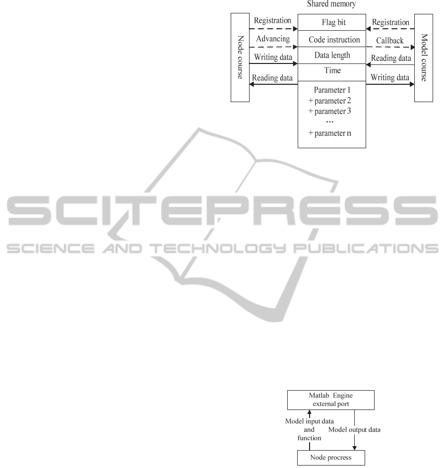
Figure 2 shows the theory of Model A driving.

Node model driving software writes data into the

shared memory based on the protocol. Models read

input data from the shared memory, and write output

data into the shared memory after operating.

The connection of model B consists of three

functions. Node model driving software drives

models by the three functions. They are initial

function, model operation control function and

reprocessing function.

Figure 2: Node model driving software and theory of

Model A driving.

To enhance the operating efficiency of simulation

platform, large of initial jobs are done in the model

initial function. 1) The platform can distribute

memory space for all the model initial /input/output

parameters. 2) The platform can find the memory

address of each model input parameter in the

structure according to the model connections. 3) The

platform can reorder the model based on the model

operation sequence. 4) The platform can drive each

initial function of models.

Model operation control function determines the

simulation cycle index based on platform simulation

step and model step. Platform drives models orderly

based on model operation sequence.

Reprocessing function invokes each reprocessing

function of models, and releases the memory space

opened before.

Figure 3: Schematic diagram of Model C driving.

Figure 3 is the schematic diagram of Model C

driving. Node model driving software brings m(mdl)

file to Matlab Engine to make calculation through

Matlab Engine external interface, then reads

computing results from Matlab Engine. In this mode,

the relationship between node model driving

software and Matlab Engine is C/S(Client/Service).

Node model driving software regarding as a

calculation servicer, through the distributed platform,

sends or receives messages to Matlab Engine. The

messages include orders and data information.

SIM-AFlexible,ScalableandExpandableSimulationPlatformApplyingtoLunarOrbitRendezvousMission

3.2 Other Function Management

Experiment management is to assemble models

taking the form of visualization, configure model

connections, distribute calculation nodes for models,

model parameters, model simulation step, simulation

condition, forming the simulation scenario.

User finishes configuring models in the form of

graphical modeling, selecting models in the form of

dragging, designing data stream in the form of

connection. It becomes the concrete simulation

experiment after assembling. Model is shown as a

rectangular module with input/output ports. User

finishes assembling models by the operation like

clicking, dragging, and connecting. On the process

of model assembling, if the input port doesn’t match

an output port, the platform will give an alarm.

Models used to be assembled come from model

library.

Distribution simulation management is designed

using the thought of “distributed calculation,

concentrated management”. One of the main goals is

distributing models and model parameters to each of

related nodes, and operating models on the node or

node computer itself in the long distance based on

the simulation scenario. Simulation scenario is its

input. After operating, user can see the operation tips

on the user interface.

Operation management includes distributed

scheduling, node supervising, simulation breakpoint

reserving. It is the foundation of simulation system

distributed operation. Operation management

program is set in the management node computer. It

can drive or distribute models on the calculation

node. At the same time, it can supervise the node

state in the long distance, and reserve the experiment

information at breakpoint.

Node management is set on the calculation node.

It is the foundation of “distributed calculation,

concentrated management”. Its main goals are node

watching, driving the model on the node and

reporting of the node state. It echoes operation

management which is set on the management node.

It drives and distributes models on the calculation

node based on the simulation scenario file, and

reports the state of local node to management node

computer.

3.3 Modelling Distributed Environment

In the process of modeling for lunar orbit rendezvous

mission, it is very important to consider the

complicated spacecraft dynamic conditions, and high

precision of the navigation and control in the close

range rendezvous phase. These factors request

sufficient accuracy of relates models. In the aspect of

modeling, program developing must obey the

standard of each type model port.

According to the requirements of the mission, we

build relative navigation model, relative SDOF

control model, thruster control assigning model, and

spacecraft relative dynamic model.

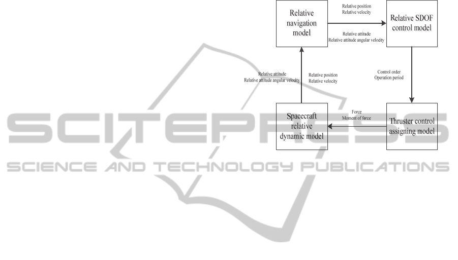
Figure 4: The information flow chart of models.

Figure 4 presents the information flow chart of

models. At the beginning of the simulation, the first

group input data is the initialization of the relative

navigation model. After filtering calculation,

measuring error is decreased, and the output data is

the relative state between the spacecrafts. The

relative state is as the input of the relative SDOF

control model, through a series of control calculation,

its output is the orders and operation period of the

thrusters. Thruster control assigning model

calculates force and moment of force based on the

thruster orders. Spacecraft relative dynamic model

inversely works out the relative state of spacecrafts

which is controlled based on the output data from the

thruster control assigning model. The relative state is

regarded as the input on the next step.

In the process of modeling, we also use the

model-templet to restrict the model ports. The above

several models are developed in the form of dynamic

link library. Model is named by capital English

acronyms XXX. Each model includes the initial

function XXX_init, Steplike function XXX_sim, and

reprocessing function XXX_end. Three functions

have the unified form. For example, the initial

function of the relative navigation model is designed

as Void RelNavigation_Init (void *pInit, void

*pInput, void *pOutput, void *pUser). It is

convenient for model management and model

driving background.

Figure 5 is the class diagram of lunar orbit

rendezvous simulation system.

SIMULTECH2015-5thInternationalConferenceonSimulationandModelingMethodologies,Technologiesand

Applications

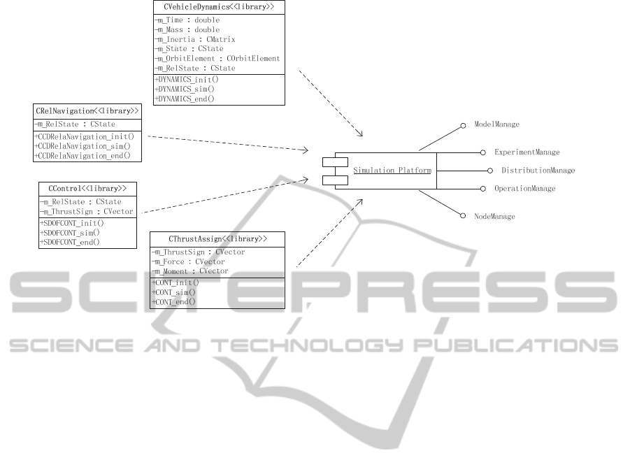
Figure 5: Class diagram of lunar orbit rendezvous simulation system.

From the class diagram, we can see that, the

whole simulation system consists of spacecraft

relative dynamic module, relative navigation module,

relative SDOF control module, and thruster control

assigning module. And, spacecraft relative dynamic

module called CVehicleDynamics includes three

functions which are DYNAMIC_init,

DYNAMIC_sim and DYNAMIC_end. Among them,

the function of DYNAMIC_sim includes many

functions referring to the basic spacecraft dynamic.

Such as coordinate system transformation,

orbital/attitude parameters transformation, spacecraft

precision orbit determination. One of the main

functions is the state transferring function which can

transfer the absolute state of the spacecrafts to the

relative state between them in the Hill coordinate. It

is easy to analyze the problems of the spacecraft

rendezvous at close range by the use of the relative

state between two spacecrafts.

One of the main goals of relative navigation

module which is named of CCDRelNavigation is

decreasing the effects of measure noise to the

docking sensor. It consists of three functions. They

are called CCDRelaNavigation_init,

CCDRelaNavigation_sim and

CCDRelaNavigation_end. Moreover,

CCDRelaNavigation_sim function encapsulates

some familiar filter methods. State transfer matrix

and state equation mentioned in the filter method are

worked out based on the spacecraft relative

orbital/attitude equations.

Relative SDOF control module and thruster

control assigning module form the chase control

section. By the use of phase plane control method,

CControl module receives navigation data,

producing control signs and bring them to

CThrustAssign module. CThrustAssign module

gives out relative state data which is after the

control.

As it is mentioned, SimulationPlatform presents

SIM simulator. It has the function of model

management, experiment management, distribution

management, operation management and node

management.

4 EXPERIMENTAL RESULTS

Making a test is a key link to verify the simulation

platform. By analyzing the results of experiment,

advantage and disadvantage of the platform and

models will be found. It is beneficial for the platform

to be developed and upgraded in the future. For

models, we can also make some significant

conclusions and found for modeling on the next step.

At the same time, experiment results are the standard

to estimate the validity of platform and models. In

this section, we make a test about lunar orbit

rendezvous simulation system.

The initialization of experiment is that target

vehicle is moving in an approximately circular orbit

around the moon. The orbit altitude is 300

kilometers. Its orbit angular velocity is 0.0007615

SIM-AFlexible,ScalableandExpandableSimulationPlatformApplyingtoLunarOrbitRendezvousMission

radian per second. The influence of the perturbative

force to vehicles is not concerned, and attitude/orbit

control motors maintain constant power. Initial

simulation parameters and initial model parameters

are set as Table 1 and Table 2.

Table 1: Initial parameters of the simulation system.

Simulation initial condition parameters

Starting time 0 s

System step 0.5 s

Step number 0

Terminal time 800 s

Current time 0 s

Model step 0.05 s

Table 2: Initial parameters of models.

Model initial condition parameters

Relative position [100, 0.01, 0.8] m

Relative velocity [-0.155, -0.07, 0.01] m/s

Relative attitude angle [2, 2, 2] deg

Relative attitude angle velocity [0.02, 0.04, 0.02] deg/s

chase vehicle moment of inertia

[7285.46, 0.00, 0.00; 0.00, 6666.67, 0.00; 0.00, 0.00, 3285.47]

target vehicle moment of inertia

[7000.00, 0.00, 0.00; 0.00, 7000.00, 0.00; 0.00, 0.00, 5000.00]

chase vehicle mass 4000 kg

chase vehicle size [1, 0, 0] m

Thruster force arm [2.00, 2.00, 1.21] m

Position of the chase vehicle docking interface [0.50, 2.00, 1.21] m

Position of the target vehicle docking interface [0.50, 2.00, 1.21] m

Force of the orbit thruster [25.00, 25.00, 25.00] N

Force of the attitude thruster [10.00, 10.00, 10.00] N

Installation position of CCD camera [1.00, 0.00, 0.00]

Viewing angle of CCD camera [6, 6] deg

Viewing point of CCD camera 30 m

Position of mooring 30 m

Milestone of velocity 60 m

Mooring time 300 s

X position error(short/long range) [0.02, 0.006; 0.15, 0.005] m

Y/Z position error(S/L range) [0.02, 0.005; 0.2, 0.004] m

Vx error(S/L range) [0.01, 0.006; 0.15, 0.01] m/s

Vy/Vz error(S/L range) [0.01, 0.01; 0.2, 0.018] m/s

X attitude angle error(S/L range) [0.23; 0.3] deg

Y/Z attitude angle error (S/L range) [0.25; 0.3] deg

x attitude angle velocity (S/L range) [0.17, 0.012; 0.2, 0.002] deg/s

y/z attitude angle velocity (S/L range) [0.2, 0.02; 0.3, 0.005] deg/s

SIMULTECH2015-5thInternationalConferenceonSimulationandModelingMethodologies,Technologiesand

Applications

In view of the above test configuration, we make

a test. The experiment results are as follow.

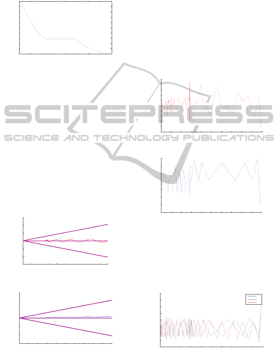
Figure 6: The X position transferring with time.

1) Figure 6 shows the X position transferring with

time. In this graph, we can see the relative

position of the two spacecrafts changing from

100 meters to 0 meter in the end. In the distance

of 30 meters, the chase vehicle stops for 300

seconds at predetermined location. The period of

the whole docking process is about 780 seconds.

Because the terminal time of simulation platform

is 800 seconds, relative position is keeping 0

meter during the last 20 seconds.

2) Figure 7-Figure 8 respectively describes the

process of relative Y/Z position changing with

the docking distance. As approaching of two

spacecrafts, the amplitude of the relative Y/Z

position is decreasing, converging to 0 meter at

last. In the process, target vehicle is staying in the

CCD detecting scope of the chase vehicle all the

time.

Figure 7: The Y position transferring with docking

distance.

Figure 8: The Z position transferring with docking

distance.

3) Figure 9-Figure 10 respectively describes the

changing process of azimuth angle and pitch

angle of CCD camera with the docking distance.

The Attitude of Chase vehicle is controlled by

impulses of attitude control engine continuously.

When the distance between two spacecrafts is

near, target vehicle is easy to deviate from the

detection scope of the chase vehicle. By the

correct flight strategy and suitable control mean,

target vehicle doesn’t deviate from the scope, but

azimuth/pitch angle is going to converge in the

range of

0.5



. It illuminates the control strategy

used in the model is available.

Figure 9: Azimuth angle of CCD camera.

Figure 10: Pitch angle of CCD camera.

4) Figure 11-Figure 12 respectively shows the

changing process of relative altitude angle and

altitude angular velocity between two spacecrafts

with the docking distance. At the end of the

docking process, relative altitude angle precision

can reach

0.5deg



, relative altitude angular

velocity precision can reach

0.1deg/



Figure 11: Relative altitude angle.

0 100 200 300 400 500 600 700 800

100

Tim e (s )

X posi ti on (m

)

0 10 20 30 40 50 60 70 80 90 100

-15

-10

-5

X position (m)

Y posi ti on (m)

0 10 20 30 40 50 60 70 80 90 100

-15

-10

-5

X position (m)

Z posi ti on (m)

0 10 20 30 40 50 60 70 80 90 100

-2.5

-2

-1.5

-1

-0.5

0.5

1.5

2.5

X position (m)

CCD Az imuth angl e



az ( deg)

0 10 20 30 40 50 60 70 80 90 100

-2

-1.5

-1

-0.5

0.5

1.5

X position (m)

CCD pi tch angl e



el (deg)

0 10 20 30 40 50 60 70 80 90 100

-1.5

-1

-0.5

0.5

1.5

2.5

X position (m)

Attitude angle







(°)







SIM-AFlexible,ScalableandExpandableSimulationPlatformApplyingtoLunarOrbitRendezvousMission

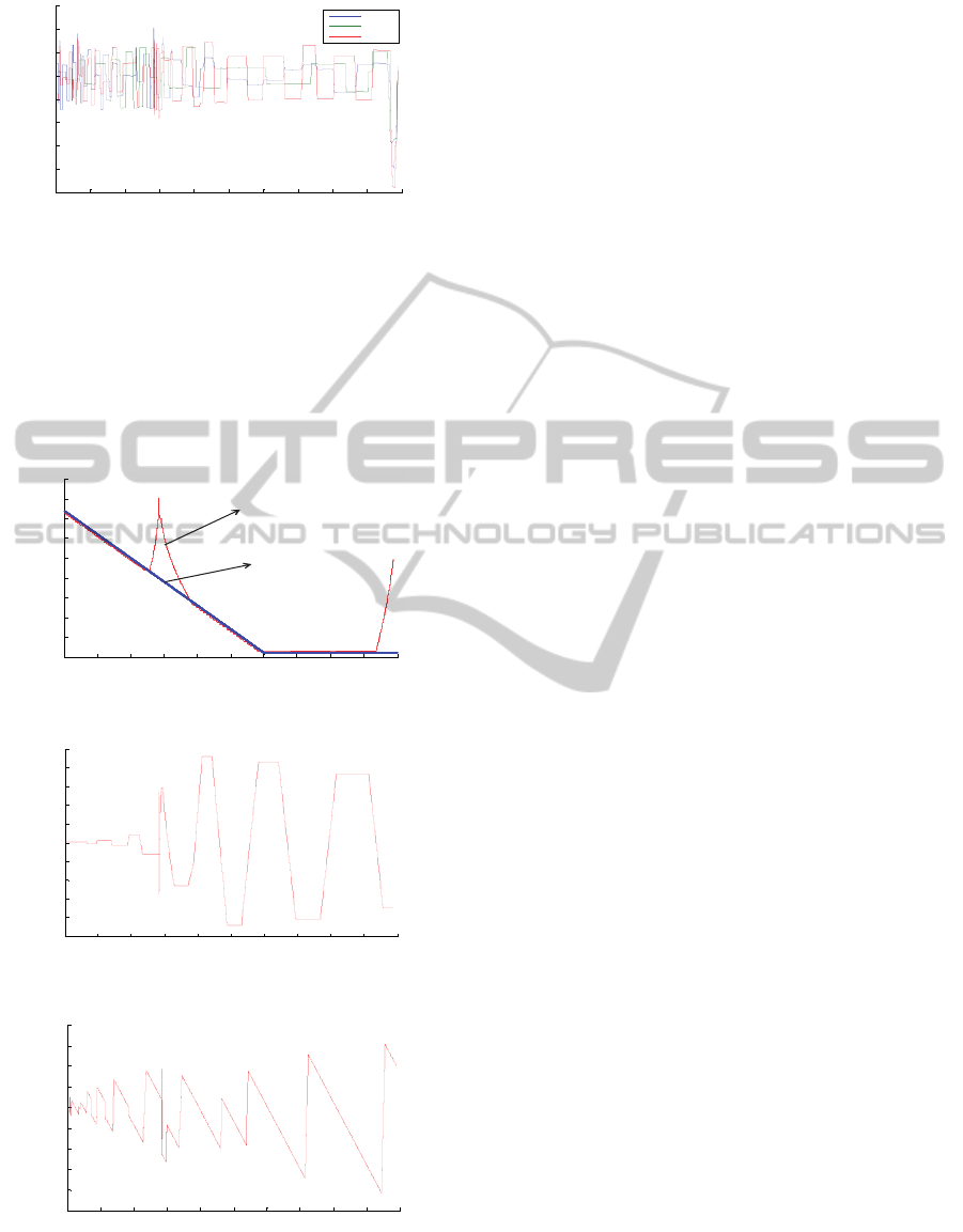
Figure 12: Altitude angular velocity.

5) Figure 13-Figure 15 respectively shows the

changing process of velocity between two

spacecrafts with the docking distance. At the end

of the docking process, the relative velocity

precision can be controlled in the range of

0.05 /ms

which meets the requirements of

spacecraft docking velocity.

Figure 13: Changing process of Vx.

Figure 14: Changing process of Vy.

Figure 15: Changing process of Vz.

5 CONCLUSIONS

In this paper we present a modelling and simulation

platform called SIM, which aims towards the study

of parallel applications on distributed systems. This

platform eases the process of designing and testing

both the applications and the architectures.

The features of this platform are as follows. First,

a great level of flexibility that allows modelling a

wide range of designs is presented. Second, a

friendly user interface, which helps to design the

experiment and look for the architecture limits and

bottlenecks is shown. Finally, the most important

feature is a good separation between the platform

and models which decreases much trouble in the

process of system assembling.

The platform presents a modular design where

the main components are the basic systems of

distributed architecture such as computing, memory,

storage, and network. This design also follows a

hierarchical philosophy, where basic modules are

grouped to compose bigger modules. SIM also

provides several modules to simulate different

components, and modeling strategies. Furthermore,

the system allows the implementation of new

modules by using a standardized interface.

Moreover, a series of models aon lunar orbit

rendezvous has been performed. Relative navigation

model, relative SDOF control model, thruster control

assigning model, and spacecraft relative dynamic

model have been configured and executed in SIM.

Our platform shows very good result in the level

of accuracy and performance obtained.

Future works on increasing the functionality of

SIM are as following. First, a tool for modeling

design and compiling. Second, encapsulation and

decapsulation design for experiment models. Third,

applying to multiple middleware protocols. Finally,

accumulating and developing models. In the above

case, we can lay the foundation of the manned lunar

landing mission next step.

REFERENCES

Bocam K. J, Brown C. M., Nelson D. K., et al., 2005. A

Space Exploration Architecture for Human Lunar

Missions and Beyond. 1st Space Exploration

Conference: Continuing the Voyage of Discovery 30

January-1 February 2005, Orlando, Florida.

Santovincenzo A., 2004. Architecture Study for

Sustainable Lunar Exploration. ESA CDF Study

Report.

0 10 20 30 40 50 60 70 80 90 100

-0.5

-0.4

-0.3

-0.2

-0.1

0.1

0.2

0.3

X position (m)

At t it ude angular vel ocit y\dphi ,dt heta, dpsi (°/ s)

dphi

dtheta

dpsi

0 10 20 30 40 50 60 70 80 90 100

-0.4

-0.35

-0.3

-0.25

-0.2

-0.15

-0.1

-0.05

0.05

X position

(

)

Vx ( m/s

)

The actual curve

The curve without berthing

0 10 20 30 40 50 60 70 80 90 100

-0.1

-0.08

-0.06

-0.04

-0.02

0.02

0.04

0.06

0.08

0.1

X position (m)

Vy (m/s)

0 10 20 30 40 50 60 70 80 90 100

-0.025

-0.02

-0.015

-0.01

-0.005

0.005

0.01

0.015

0.02

X position (m)

Vz (m/s)

SIMULTECH2015-5thInternationalConferenceonSimulationandModelingMethodologies,Technologiesand

Applications

Reeves D. M., 2005. The Apollo Lunar Orbit Rendezvous

Architecture Decision Revisited. AIAA 2005-4011.

Raftery M., Fox T., 2007. The Crew Exploration Vehicle

(CEV) and the Next Generation of Human Spaceflight.

Acta Astronautica.

Argollo E., A. Falcon, Faraboschi P., Monchiero M.,

Ortega D., 2009. COTSon: infrastructure for full

system simulation, SIGOPS Operating Systems,

Review 43 (1) (2009) 52–61.

Binkert N. L., Dreslinski R. G., Hsu L. R., Lim K. T.,

Saidi A.G., Reinhardt S.K., 2006. The M5 simulator:

modeling networked systems, IEEE Micro 26 (4) (2006)

52–60.

Magnusson P., Christensson M., Eskilson J., Forsgren D.,

Hallberg G., Hogberg J., Larsson F., Moestedt A.,

Werner B., 2002. Simics: a full system simulation

platform, Computer 35 (2) (2002) 50–58.

Rosenblum M., Herrod S. A., Witchel E., Gupta A., 1995.

Complete computer system simulation: the SimOS

approach, Parallel & Distributed Technology: Systems

& Applications, IEEE 3 (4) (1995) 34–43.

Rosenblum M., Bugnion E., Devine S., Herrod S. A., 1997.

Using the SimOS machine simulator to study complex

computer systems, ACM Transactions on Modeling

and Computer Simulation 7 (1) (1997) 78–103.

Zhai J., Chen W., Zheng W., 2010. PHANTOM: predicting

performance of parallel applications on large-scale

parallel machines using a single node, in: PPoPP’10:

Proceedings of the 15th ACM SIGPLAN Symposium

on Principles and Practice of Parallel Programming,

ACM, New York, NY, USA, 2010, pp. 305–314.

Cornea B., Bourgeois J., 2010. Simulation of a P2P

parallel computing environment–introducing dPerf, a

tool for predicting the performance of parallel MPI or

P2P-SAP applications, Technical Report RT2010-04,

LIFC–Laboratoire d’Informatique de l’Universite de

Franche Comte, March 2010.

Liao C., Quinlan D. J., Vuduc R. W., Panas T., 2009.

Effective source-to-source outlining to support whole

program empirical optimization, in: LCPC’09: 22

International Workshop on Languages and Compilers

for Parallel Computing, 2009, pp. 308–322.

Tarapore S., Smullen C., Gurumurthi S., 2008. MIDAS: An

execution-driven simulator for active storage

architectures, in: Workshop on Modeling,

Benchmarking, and Simulation (Held in Conjunction

with ISCA 2008), Beijing, China, 2008, pp. 1–10.

SIM-AFlexible,ScalableandExpandableSimulationPlatformApplyingtoLunarOrbitRendezvousMission