
Kinematic Analysis and Simulation of a Hybrid Biped Climbing Robot
Adri
´
an Peidr
´
o, Arturo Gil, Jos
´
e Mar
´
ıa Mar
´
ın, Yerai Berenguer and
´
Oscar Reinoso
Systems Engineering and Automation Department, Miguel Hern
´
andez University, 03202, Elche, Spain
Keywords:
Biped Robots, Climbing Robots, Hybrid Serial-parallel Robots, Kinematics, Redundant Robots, Simulation.
Abstract:
This paper presents a novel climbing robot that explores 3-D truss structures for maintenance and inspection
tasks. The robot is biped and has a hybrid serial-parallel architecture since each leg is composed of two
parallel mechanisms connected in series. First, the forward kinematic problem of the complete robot is solved,
obtaining the relative position and orientation between the feet in terms of the ten joint coordinates of the
robot. The inverse kinematics is more complex due to the redundancy of the robot. Hence, a simplified inverse
kinematic problem that assumes planar and symmetric movements is analyzed. Then, a tool to simulate the
kinematics of the robot is presented, and it is used to demonstrate that the robot can completely explore 3-D
structures, even when some movements are restricted to be planar and symmetric.
1 INTRODUCTION
Vertical structures such as buildings, bridges, silos,
or towers require periodic maintenance and inspec-
tion operations. For example, the glass facades of
skyscrapers must be cleaned, and the welded unions
in the metallic skeletons of the buildings must be ex-
amined. Tasks like these are very dangerous for hu-
man operators, who must work in environments of-
ten difficult to access and are exposed to many risks
such as falling from height, contamination (e.g. in-
spections in nuclear or chemical facilities) or elec-
trocution (e.g. maintenance of power transmission
lines). To eliminate these risks, during the last two
decades many researchers have been investigating the
possibility of automating the execution of these tasks
using climbing robots. (Schmidt and Berns, 2013)
present an exhaustive analysis of the applications and
design criteria of climbing robots, as well as a com-
prehensive review of the main locomotion and adhe-
sion technologies.
Three-dimensional truss structures are present in
many vertical structures such as bridges, towers and
skeletons of buildings. These structures are typically
constituted by a network of beams connected at struc-
tural nodes, and a high degree of mobility is often
required to explore them. Climbing robots for 3-D
trusses can be classified into two main types (Tavakoli
et al., 2011): continuous-motion and step-by-step
robots. Continuous-motion robots are faster, use
wheels, and employ magnetism or friction to adhere
to the structure (Baghani et al., 2005; Tavakoli et al.,
2013). However, they usually have more difficul-
ties to negotiate obstacles and their wheels may slip.
Step-by-step robots have two grippers connected by a
kinematic chain which has some degrees of freedom
(DOF). Their name reflects their locomotion method:
in each motion cycle, one gripper is fixed to the struc-
ture, whereas the kinematic chain moves the other
gripper to the next attachment point of the structure,
where it will be fixed. Then, the previously fixed grip-
per is released and a new motion cycle begins. During
each motion cycle, these robots are equivalent to typ-
ical robot manipulators. Hence, they have a higher
mobility that facilitates the avoidance of obstacles,
but they are heavier, slower, and more complex.
The architecture of the kinematic chain of step-
by-step robots can be serial, parallel, or hybrid. Se-
rial architectures have larger workspaces than parallel
ones, but they are less rigid and have a limited load
capacity. The serial architectures have been the most
explored ones in step-by-step climbing robots, with
many different designs proposed by different authors.
For example, (Balaguer et al., 2000) present a 6-DOF
robot to explore 3-D metallic structures. Since the
robot is powered by a battery, the movements are opti-
mized to reduce the energy consumption and increase
its autonomy. Another 4-DOF serial climbing robot
is presented in (Tavakoli et al., 2011). Other authors
propose serial architectures inspired by inchworms,
with 5 and 8 DOF (Guan et al., 2011; Shvalb et al.,
2013). (Mampel et al., 2009) propose a similar mod-
24
Peidro A., Gil A., Marin J., Berenguer Y. and Reinoso O..
Kinematic Analysis and Simulation of a Hybrid Biped Climbing Robot.
DOI: 10.5220/0005515800240034
In Proceedings of the 12th International Conference on Informatics in Control, Automation and Robotics (ICINCO-2015), pages 24-34
ISBN: 978-989-758-123-6
Copyright
c
2015 SCITEPRESS (Science and Technology Publications, Lda.)

ular robot whose number of DOF can be increased
connecting more modules in series. Finally, (Yoon
and Rus, 2007) present 3-DOF robots that can indi-
vidually explore 3-D trusses or can be combined with
other robots to form more complex kinematic chains
with higher maneuverability.
Parallel climbing robots are less common, but they
have also been studied. These architectures offer a
higher payload-to-weight ratio than serial robots, but
their workspace is more limited. (Aracil et al., 2006)
propose using a Gough-Stewart platform as the main
body of a robot for climbing truss structures, pipelines
and palm trees. The robot remains fixed to the struc-
ture using grippers or embracing it with its annular
platforms.
Finally, hybrid climbing robots are composed of
some serially connected parallel mechanisms, and
they have the advantages of both architectures: high
maneuverability, rigidity and load capacity. A hy-
brid robot for climbing 3-D structures is proposed
by (Tavakoli et al., 2005), who combine a 3-RPR par-
allel robot with a rotation module connected in series.
Another hybrid robot is proposed in (Figliolini et al.,
2010). In this case, the robot is biped and each leg is
the serial combination of two 3-RPS parallel robots.
Hence, the complete robot has 12 DOF.
In this paper, we present a novel 10-DOF redun-
dant hybrid robot for climbing 3-D truss structures.
The robot is biped and its legs are connected to a hip
through revolute joints. Each leg is the serial combi-
nation of two parallel mechanisms that possess linear
hydraulic actuators, which provide a high load capac-
ity and stiffness. The design of the robot makes it
specially suitable to maneuver in 3-D truss structures
and perform transitions between planes with different
orientations. In this paper, we focus on the forward
and inverse kinematic problems of the robot, which
are necessary to plan trajectories in 3-D structures.
We also present a Java simulation tool that allows us
to verify the kinematic models obtained in this paper
and demonstrate the ability of the robot to explore 3-
D trusses.
This paper is organized as follows. The architec-
ture of the robot is described in detail in Section 2.
Next, the forward kinematic problem of the complete
robot when one foot remains fixed is solved in Sec-
tion 3. In Section 4, a simplified yet useful version
of the inverse kinematic problem is solved. Then,
Section 5 presents a tool that simulates the forward
kinematics of the robot. This tool is used to demon-
strate the execution of some example trajectories by
the robot in a 3-D structure. Finally, the conclusions
and future work are exposed in Section 6.
2 DESCRIPTION OF THE ROBOT
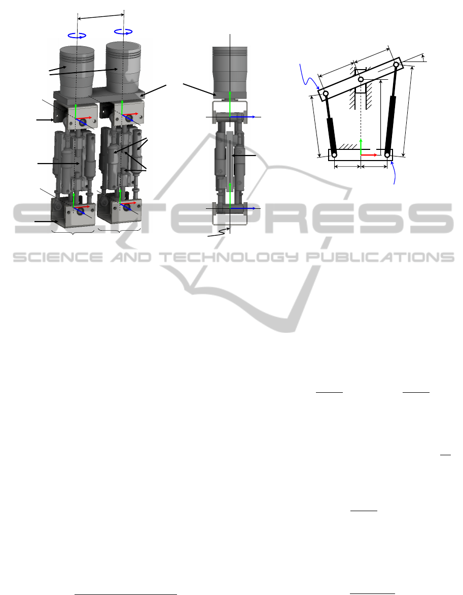
Figure 1a shows a 3-D model of the biped climbing
robot. The robot has two identical legs (A and B)
connected to the hip through revolute joints driven by
motors (angles θ
A
and θ
B
). Each leg has three links:
a core link and two platforms. The lower platform is
the foot of the leg and carries the gripper that fixes
the robot to the structure (the grippers are not consid-
ered in the kinematic analysis presented in this paper).
The upper platform is connected to the hip through
the aforementioned revolute joint. Each platform is
connected to the core link by means of two prismatic
actuators and a passive slider.
The mechanism composed of the core link, one
platform, and the two prismatic actuators that con-
nect these two elements, is a closed-loop linkage that
will be called hereafter “parallel module”. The paral-
lel modules are planar mechanisms that can be repre-
sented schematically as shown in Figure 1b. Hence,
each leg is the serial combination of the parallel mod-
ules 1 (which is connected to the foot) and 2 (which is
connected to the hip). The prismatic actuators of each
parallel module lie in opposite sides of the plane Π
j
,
which is one of the planes of symmetry of the core
link of the leg j (see the side view in Figure 1a). This
is indicated with dashed lines in Figure 2.
Figure 1a also shows some reference frames at-
tached to different parts of the robot. In this paper,
the X, Y , and Z axes of reference frames will be rep-
resented in red, green, and blue colors, respectively.
The frames H
A
and H
B
are fixed to the hip of the robot,
whereas the frames A and B are respectively attached
to the feet of the legs A and B.
The robot has 10 DOF: the rotation angles θ
A
and
θ
B
, and the four prismatic actuators of each leg. In
the next sections, the forward and inverse kinematic
problems of the robot will be analyzed. After that, we
will simulate the forward kinematics to demonstrate
its ability to explore 3-D structures.
3 FORWARD KINEMATICS
In this section, the forward kinematic problem (FKP)
of the robot is solved. The problem considered here
consists in calculating the position and orientation of
one foot with respect to the other foot when the joint
coordinates are known: the angles θ
A
and θ
B
and the
lengths (l
ij
,r
ij
) of the linear actuators of the parallel
modules (i ∈
{
1,2
}
, j ∈
{
A,B
}
). First, the forward
kinematics of the parallel modules is analyzed.
KinematicAnalysisandSimulationofaHybridBipedClimbingRobot
25
hip
θ
A
θ
B
t
upper
platform
lower
platform
(foot)
motors
H
A
H
B
A
B
leg A
leg B
core
link
prismatic
actuators
passive
sliders
Side view
plane Π
core
link
A
H
A
(a)
φ
ij
p
p
b
b
y
ij
r
ij
l
ij
X
Y
base
(attached to the core
link of the leg j)
platform
(b)
Figure 1: (a) 3-D model of the climbing robot. (b) A schematic diagram of a parallel module.
3.1 FKP of the Parallel Modules
Figure 1b shows the i-th parallel module of the leg j
(i ∈
{
1,2
}
, j ∈
{
A,B
}
). A parallel module is a closed-
loop planar mechanism composed of a mobile plat-
form connected to a base through two prismatic ac-
tuators with lengths l
ij
and r
ij
. The platform is con-
strained to only translate vertically and rotate. The
forward kinematics consists in calculating the posi-
tion y
ij
and the orientation ϕ
ij
of the mobile platform
in terms of l
ij
and r
ij
. According to Figure 1b, the
relationship between (l
ij
,r
ij
) and (y
ij
,ϕ
ij
) is:
(pcos ϕ
ij
−b)
2
+ (y
ij
+ p sin ϕ
ij
)
2
= r
2
ij
(1)
(pcos ϕ
ij
−b)
2
+ (y
ij
−p sin ϕ
ij
)
2
= l
2
ij
(2)
These equations can be combined to obtain an equiv-
alent system. Adding together Eqs. (1) and (2) yields
Eq. (3), whereas subtracting Eq. (2) from Eq. (1) re-
sults in Eq. (4):
4bpcos ϕ
ij
= 2y
2
ij
+ 2b
2
+ 2p
2
−l
2
ij
−r
2
ij
(3)
4y
ij
psinϕ
ij
= r
2
ij
−l
2
ij
(4)
Solving cosϕ
ij
from Eq. (3) gives:
cosϕ
ij
=
2y
2
ij
+ 2b
2
+ 2p
2
−l
2
ij
−r
2
ij
4bp
(5)
Squaring Eq. (4):
16y
2
ij
p
2
(1 −cos
2
ϕ
ij
) = (r
2
ij
−l
2
ij
)
2
(6)
Finally, substituting Eq. (5) into Eq. (6) yields a cubic
equation in ϒ
ij
= y
2
ij
:
ϒ
3
ij
+ k
ij
2
ϒ
2
ij
+ k
ij
1
ϒ
ij
+ k
ij
0
= 0 (7)
where:
k
ij
2
= 2b
2
+ 2p
2
−l
2
ij
−r
2
ij
(8)
k
ij
1
=
"
(b + p)
2
−
l
2
ij
+ r
2
ij
2
#"
(b − p)
2
−
l
2
ij
+ r
2
ij
2
#
(9)
k
ij
0
= b
2
(l
ij
+ r
ij
)
2
(l
ij
−r
ij
)
2
/4 (10)
Equation (7) always has three roots, two of which may
be complex. For a given strictly positive root ϒ
ij
of
Eq. (7), two solutions are obtained for y
ij
= ±
p
ϒ
ij
.
For each of these two values of y
ij
, cos ϕ
ij
is calculated
from Eq. (5), whereas sin ϕ
ij
is obtained from Eq. (4):
sinϕ
ij
=
r
2
ij
−l
2
ij
4y
ij
p
(11)
Once cos ϕ
ij
and sin ϕ
ij
are known, ϕ
ij
is unequivo-
cally determined in (−π,π]. If ϒ
ij
= 0, then y
ij
= 0 and
cosϕ
ij
is calculated using Eq. (5). However, sin ϕ
ij
cannot be calculated from Eq. (11) since y
ij
= 0. In-
stead, sinϕ
ij
is calculated as follows:
sinϕ
ij
= ±
q
1 −cos
2
ϕ
ij
(12)
obtaining two solutions. It is shown in (Kong and
Gosselin, 2002), using Sturm’s Theorem, that Eq. (7)
ICINCO2015-12thInternationalConferenceonInformaticsinControl,AutomationandRobotics
26
cannot have more than two non-negative roots. Since
each non-negative root of Eq. (7) yields two different
pairs (y
ij
,ϕ
ij
), the FKP of each parallel module has
four solutions at most.
Note that swapping the values of r
ij
and l
ij
neither
affects Eq. (7) nor Eq. (5), but it changes the sign of
sinϕ
ij
in Eq. (11). Hence, swapping r
ij
and l
ij
changes
the sign of ϕ
ij
, leaving y
ij
unchanged. This can be
observed in Figure 1b, where swapping r
ij
and l
ij
is
equivalent to rotating the figure π rad about the verti-
cal Y axis. This fact will be exploited in Section 4 to
analyze the inverse kinematics of the robot.
3.2 FKP of the Complete Robot
The forward kinematics of the complete robot con-
sists in calculating the position and orientation of
one foot with respect to the other foot when the ten
joint coordinates are known. The problem will be
solved using Homogeneous Transformation Matrices
(HTMs). An HTM has the following form (Bajd et al.,
2013):
T
m/n
=
R
m/n
t
m/n
0
1×3
1
(13)
where 0
1×3
= [0,0,0]. The matrix T
m/n
encodes the
position and orientation of a frame m with respect to
another frame n. Indeed, R
m/n
∈ R
3×3
is a rotation
matrix whose columns are the vectors of the frame m
expressed in the basis formed by the vectors of the
frame n, whereas t
m/n
∈ R
3×1
is the position of the
origin of the frame m in coordinates of the frame n.
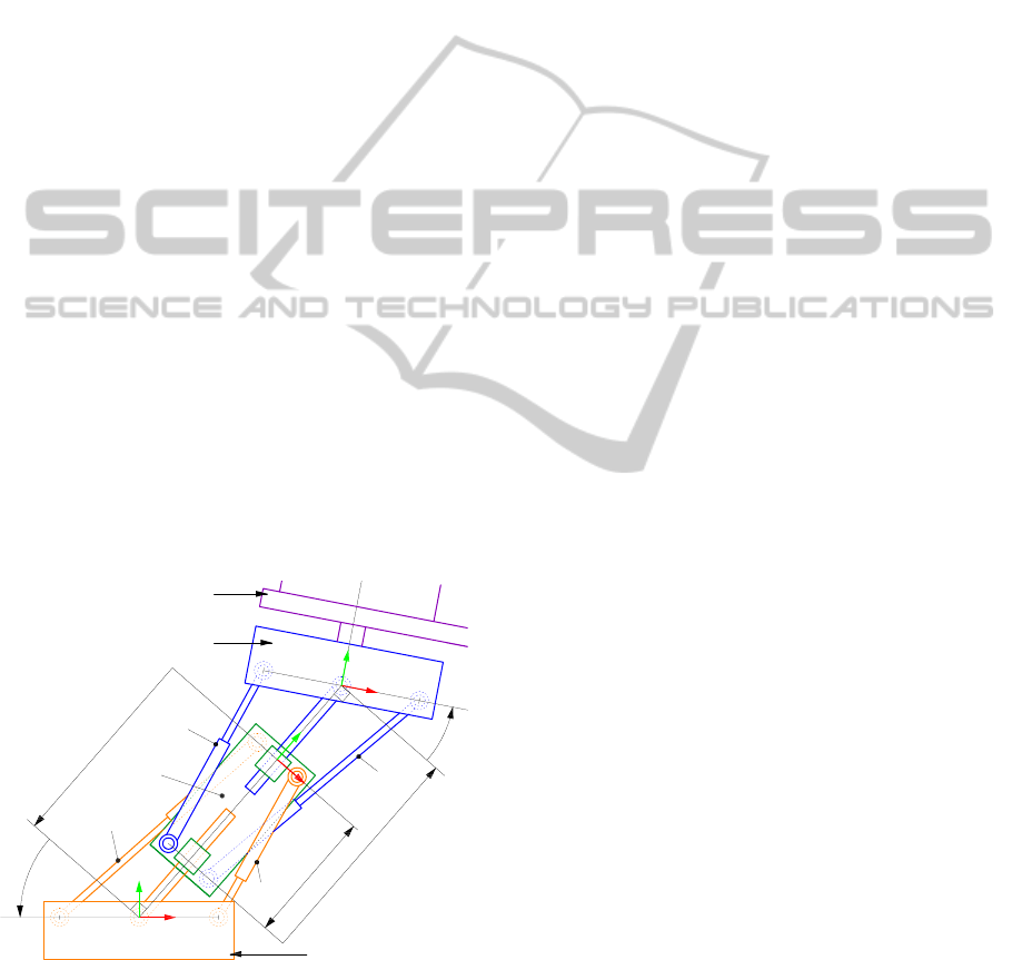
y
1j
φ
2j
h
φ
1j
core
link
j
F
j
hip
platform of the parallel
module 2
l
2j
l
1j
r
2j
r
1j
platform of the
parallel module 1
y
2j
G
j
Figure 2: Kinematics of a generic leg j ∈
{
A,B
}
.
The forward kinematics of one leg can be easily
solved using HTMs. Figure 2 represents schemati-
cally a generic leg j ∈
{
A,B
}
. Each leg has two paral-
lel modules whose bases are attached to the core link.
The platform of the parallel module 1 is the foot of
the leg, whereas the platform of the parallel module
2 is connected to the hip of the robot by means of
a revolute joint. The variables (y
1 j
,ϕ
1 j
,y
2 j
,ϕ
2 j
) are
obtained from (l
1 j
,r
1 j
,l
2 j
,r
2 j
) as explained in Sec-
tion 3.1. All the reference frames of Figure 2 are con-
tained in the plane Π
j
, which is one of the planes of
symmetry of the core link of the leg j (see Figure 1a).
The transformation between the frame j (fixed to the
foot) and the frame F
j
(fixed to the core link) is:
T
F
j
/ j
=
cosϕ
1 j
sinϕ
1 j
0 y
1 j
sinϕ
1 j
−sinϕ
1 j
cosϕ
1 j
0 y
1 j
cosϕ
1 j
0 0 1 0
0 0 0 1
(14)
Similarly, the transformation between the frame G
j
(attached to the platform of the parallel module 2) and
the frame F
j
is:
T
G
j
/F
j
=
cosϕ
2 j
−sinϕ
2 j
0 0
sinϕ
2 j
cosϕ
2 j
0 y
2 j
−h
0 0 1 0
0 0 0 1
(15)
where h is a geometric constant. Finally, a rotation θ
j
about the Y axis of the frame G
j
transforms it into the
frame H
j
, which is attached to the hip of the robot:
T
H
j
/G
j
=
cosθ
j
0 sinθ
j
0
0 1 0 0
−sinθ
j
0 cosθ
j
0
0 0 0 1
(16)
The position and orientation of the frame H
j
with re-
spect to the frame j is obtained as follows:
T
H
j
/ j
= T
F
j
/ j
T
G
j
/F
j
T
H
j
/G
j
(17)
which completes the FKP of any generic leg j. Once
the forward kinematics of each leg is solved, it is
straightforward to calculate the position and orienta-
tion of the foot of one leg k ∈
{
A,B
}
\
{
j
}
with respect
to the foot of the other leg j:
T
k/ j
= T
H
j
/ j
T
H
k
/H
j
T
k/H
k
(18)
where T
k/H
k
=
T
H
k
/k
−1
and T
H
k
/H
j
is the HTM that
encodes the position and orientation of the frame H
k
with respect to the frame H
j
:
T
H
k
/H
j
=
I t
H
k
/H
j
0
1×3
1
(19)
which is constant because both frames are attached to
the same rigid body (the hip). I is the 3 ×3 identity
matrix. Moreover, according to Figure 1a: t
H
B
/H
A
=
[t,0,0]
T
= −t
H
A
/H
B
, where t is the distance between
the parallel axes of the revolute actuators.
Note that, in theory, there are 4
4
= 256 different
solutions to the FKP of the complete robot. This is
because the kinematic chain between the feet has four
parallel modules connected in series and the FKP of
each module has four real solutions at most.
KinematicAnalysisandSimulationofaHybridBipedClimbingRobot
27

4 INVERSE KINEMATICS
The inverse kinematic problem (IKP) consists in cal-
culating the values of the joint coordinates necessary
to attain a desired relative position and orientation be-
tween the feet of the robot, and it is necessary for
planning trajectories. In this robot, ten joint coordi-
nates are used to place and orient one foot with respect
to the other foot, which makes it redundant. Hence,
the IKP is underconstrained and one should expect
infinitely many solutions. This redundancy makes it
difficult to solve the general IKP of this robot. For-
tunately, many important movements necessary to ex-
plore a 3-D structure (e.g., walking in one dimension,
changing between planes, etc) can be executed using
the configuration analyzed in this section, which re-
duces the number of variables and simplifies remark-
ably the IKP.
j
G
j
ω
µ
L
t/2
G
k
k
X
Y
X
X
X
Y
Y
Y
leg j
leg k
Figure 3: The Planar Symmetric Inverse Kinematic (PSIK)
problem.
The configuration considered in this section is de-
picted in Figure 3, where the foot j is fixed to the
structure and the foot k is mobile ( j,k ∈{A,B}, j 6= k).
It is assumed that the Z axes of the frames attached to
the feet are parallel and point in the same direction.
Hence, any variation in the length of the prismatic ac-
tuators of the parallel modules only produces planar
motions of the frame k in the XY plane of the frame j.
In this case, the position and orientation of the frame
k relative to the frame j can be calculated as follows:
T
k/ j
= T
G
j
/ j
I [t,0,0]
T
0
1×3
1
T
G
k
/k
−1
(20)
where T
G
j
/ j
= T
F
j
/ j
T
G
j
/F
j
. Moreover, it is assumed
that the joint coordinates of the parallel modules of
the two legs are related as follows:
l
ik
= r
ij
, r
ik
= l
ij
(i = 1, 2) (21)
This means that the joint coordinates of the parallel
module i of the legs k and j are swapped. According
to Section 3.1, this translates into:
y
ik
= y
ij
, ϕ
ik
= −ϕ
ij
(i = 1, 2) (22)
It can be graphically checked that Eq. (22) implies
that the legs k and j are symmetric with respect to the
line L, which is the axis of symmetry of the hip of the
robot. Substituting Eq. (22) into Eq. (20), the matrix
T
k/ j
can be written only in terms of the variables of
the leg j and has the following expression:
T
k/ j
=
−c(2ω) −s(2ω) 0 µ(1 −c(2ω))
s(2ω) −c(2ω) 0 µ ·s(2ω)
0 0 1 0
0 0 0 1
(23)
where s(x) = sin x, c(x) = cos x and:
µ =
t −2(h −y
1 j
−y
2 j
)sinϕ
2 j
2cos(ϕ
1 j
−ϕ
2 j
)
(24)
ω = ϕ
1 j
−ϕ
2 j
+ π/2 (25)
Thus, under the condition of planar and symmetric
motion, the position and orientation of the foot k rel-
ative to the foot j can be defined by two parame-
ters (µ, ω), which are indicated in Figure 3. We de-
fine the Planar Symmetric Inverse Kinematic (PSIK)
problem, which consists in calculating the joint co-
ordinates (l
1 j
,r
1 j
,l
2 j
,r
2 j
) needed to achieve a desired
position and orientation (µ,ω). Since the joint coor-
dinates do not appear explicitly in Eqs. (24)-(25), the
kinematic equations of the parallel modules of the leg
j must be included:
(p cos ϕ
1 j
−b)
2
+ (y
1 j
+ p sin ϕ
1 j
)
2
= r
2
1 j
(26)
(p cos ϕ
1 j
−b)
2
+ (y
1 j
−p sin ϕ
1 j
)
2
= l
2
1 j
(27)
(p cos ϕ
2 j
−b)
2
+ (y
2 j
+ p sin ϕ
2 j
)
2
= r
2
2 j
(28)
(p cos ϕ
2 j
−b)
2
+ (y
2 j
−p sin ϕ
2 j
)
2
= l
2
2 j
(29)
Hence, the PSIK problem requires calculating
(l
1 j
,r
1 j
,l
2 j
,r
2 j
,y
1 j
,ϕ
1 j
,y
2 j
,ϕ
2 j
) from Eqs. (24)-(29).
Like the general inverse kinematic problem, the PSIK
problem is underconstrained since eight unknowns
must be obtained from six equations. However, the
PSIK problem involves less variables and simpler
equations. In the following section, we will show that
some postures necessary to negotiate obstacles in a
3-D structure can be analyzed solving the PSIK prob-
lem. Also, we will describe a method to choose ap-
propriate solutions to the PSIK problem assuming that
the lengths of the prismatic actuators of the parallel
modules have upper and lower limits.
ICINCO2015-12thInternationalConferenceonInformaticsinControl,AutomationandRobotics
28
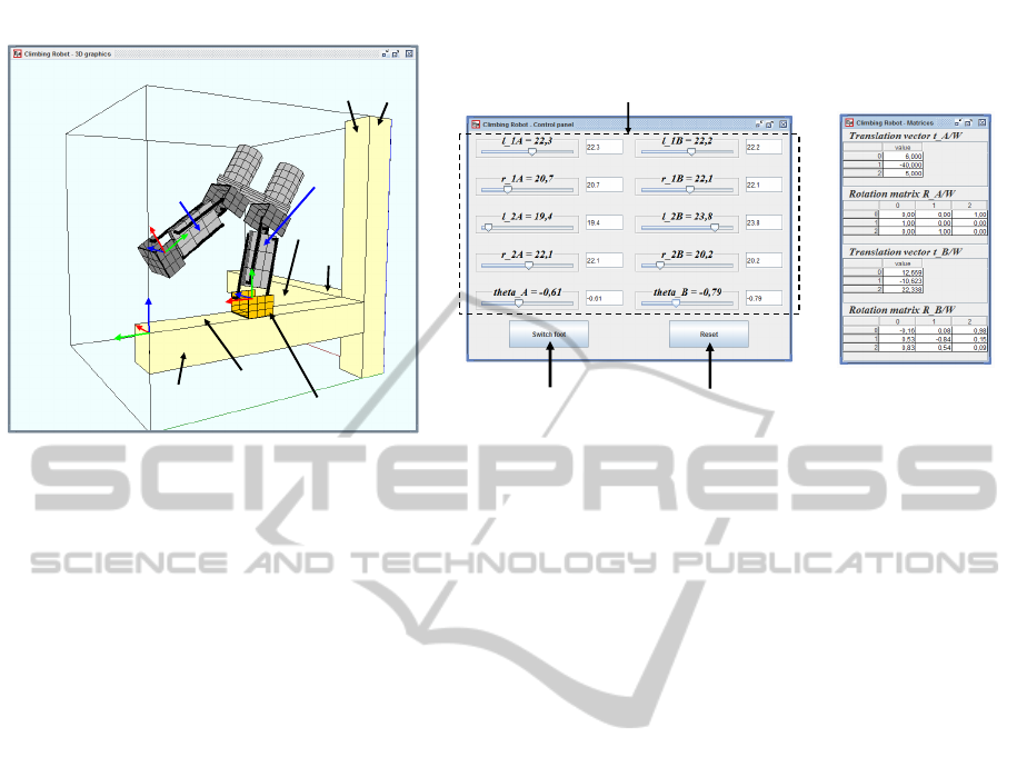
W
leg A
leg B
Graphical window
Control window
Sliders for modifying the
joint coordinates
Button for changing
the fixed foot
Button for resetting
the simulator
b
1
b
2
Fixed foot
b
3
f
1
f
4
f
2
Output
window
B
A
Figure 4: Interface of the tool developed to simulate the forward kinematics of the robot.
5 SIMULATION
In this section, we will simulate the movements of
the complete robot in an example 3-D structure to
validate the kinematic analyses of Sections 3 and 4,
and demonstrate the ability of the robot to explore
the structure. More specifically, we will show how
the robot can walk on a beam, perform transitions
between different faces of the beams, and negotiate
structural nodes.
To demonstrate these movements, we have devel-
oped a Java simulation tool that can be downloaded
from http://arvc.umh.es/parola/climber.html (the lat-
est version of Java may be required). The simula-
tor implements the equations derived in Section 3 to
solve the forward kinematics. As shown in Figure 4,
the simulator has a graphical window that shows the
robot in the 3-D test structure. The tool also has a
window with a control panel where the user can mod-
ify the values of the ten joint coordinates, change the
foot that is attached to the structure, or reset the sim-
ulation. It is important to remark that the simulation
tool only implements the kinematic equations, with-
out considering the dynamics of the robot (gravity is
neglected) or the collisions between the robot and the
structure. These advanced topics will be analyzed in
the future.
Three reference frames are shown in the graphical
window of the simulator: the world frame W (which
is attached to one of the corners of the beam b
1
of the
structure) and the frames A and B (which are attached
to the feet of the legs). The fixed foot is indicated
in orange color. When the user modifies the value of
a joint coordinate, the forward kinematics is solved
and the position and orientation of the free foot with
respect to the frame W is calculated as follows:
T
k/W
= T
j/W
T
k/ j
(30)
where the matrix T
k/ j
is defined in Section 3.2, j
denotes the fixed leg, and k denotes the mobile leg
( j,k ∈
{
A,B
}
, j 6= k). As shown in Figure 4, the trans-
lation and rotation submatrices of T
A/W
and T
B/W
are
indicated to the user in an output window of the sim-
ulator. According to Section 3.2, there are 256 solu-
tions to the forward kinematics of the complete robot
since each parallel module can have up to four dif-
ferent solutions. However, it will be shown next that
only one solution is valid.
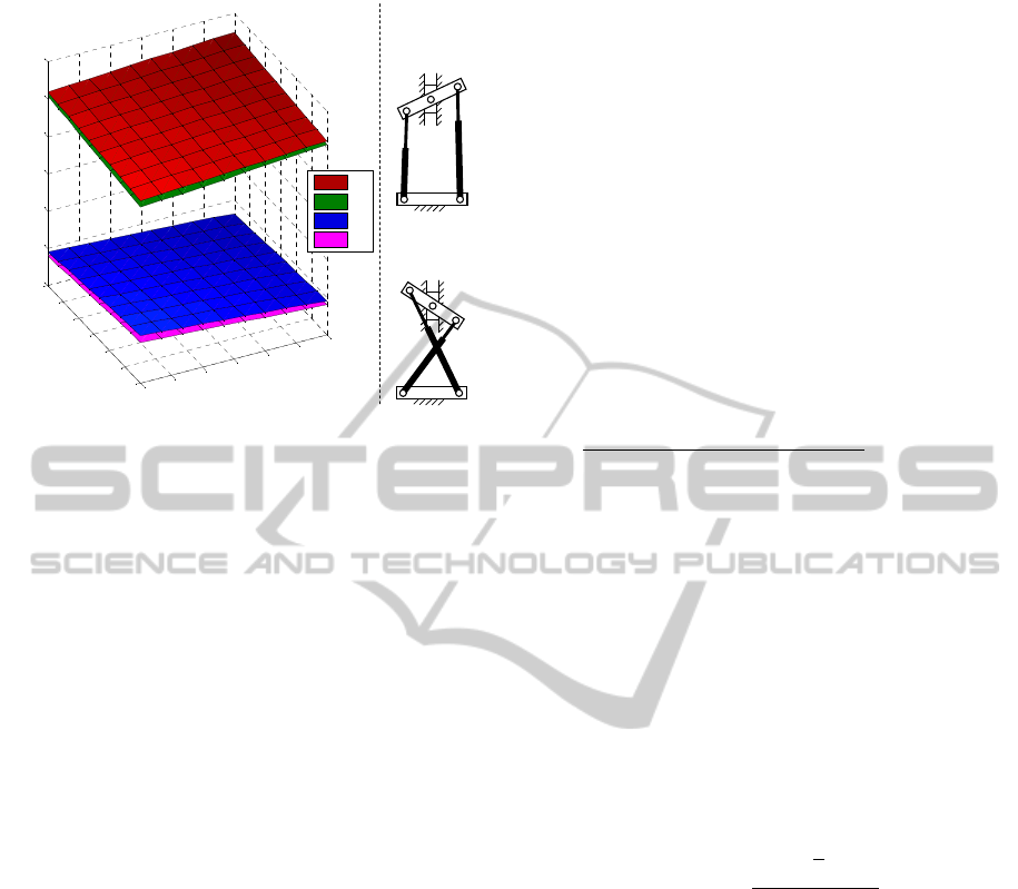
For the following simulations, we will assume
that b = p = 4 cm, and that the prismatic actuators
are constrained so that r
ij
,l
ij
∈ [19,25] cm. Solving
the forward kinematics of a parallel module for these
ranges of the joint coordinates, and plotting the solu-
tion y
ij
versus r
ij
and l
ij
, results in the four surfaces
shown in Figure 5. Each surface is associated with
one of the configurations labeled as follows: H
+
, X
+
,
H
−
, and X
−
. The solutions H
+
and X
+
are indicated
in Figure 5; the solutions H
−
and X
−
are their re-
spective mirror images with respect to the base of the
parallel module. According to the design of the robot
(see Section 2), the only valid solution is H
+
, since
the other solutions are impossible due to mechani-
cal interferences between different links of the legs.
Moreover, Figure 5 also provides a criterion for se-
lecting the valid solution: the solution H
+
always has
the highest y
ij
coordinate.
Once the only valid solution to forward kinematics
has been characterized, we will simulate the execu-
tion of an example trajectory in the structure, which is
KinematicAnalysisandSimulationofaHybridBipedClimbingRobot
29
19
20
21
22
23
24
25
19
20
21
22
23
24
25
-30
-20
-10
0
10
20
30
y
ij
(cm)
l
ij
(cm)
r
ij
(cm)
H
+
X
+
X
–
H
–
H
+
X
+
Figure 5: Solution surfaces of the FKP of a parallel module
for b = p = 4 cm. The surfaces H
+
and H
−
are almost
parallel to the surfaces X
+
and X
−
, respectively.
composed of the three beams b
1
, b
2
, and b
3
indicated
in Figure 4. At the beginning of the trajectory, the
robot lies on the face f
1
of the beam b
1
, and the objec-
tive is to move the robot to the face f
4
of the beam b
3
,
negotiating the structural node where the three beams
intersect. Next, we will show that such a trajectory
can be executed by a sequence of basic movements
that can be used to reach any other point of the struc-
ture. The values of the remaining geometric parame-
ters of the robot are: t = 15.6 cm, h = 16 cm. More-
over, the side of the square cross section of the beams
measures 12 cm, and the distance between the face f
2
of the beam b
2
and the origin of the frame W is 88 cm.
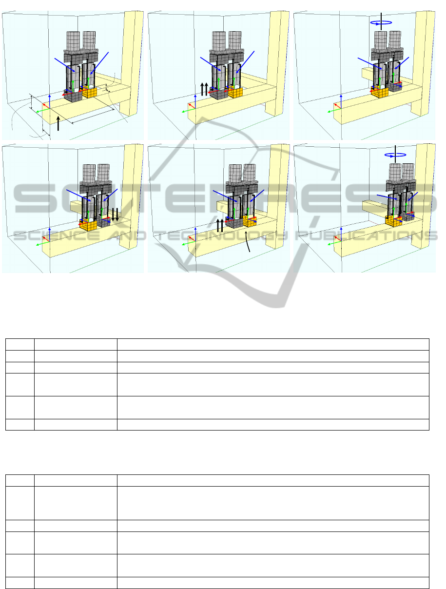
5.1 Phase 1: Walking Along a Beam
At the beginning of the trajectory (see Figure 6a), the
foot A is attached to the face f
1
of the beam b
1
, and the
frame A has the following position and orientation:
t
A/W
=
6
−40
5
cm, R
A/W
=
0 0 1
1 0 0
0 1 0
(31)
The number “6” in t
A/W
means that the frame A is
centered in the beam, whereas the number “5” is
a geometric constant of the feet of the robot. Ini-
tially, the joint coordinates have the following values:
θ
A
= θ
B
= 0, r
ij
= l
ij
= 21 cm (i ∈
{
1,2
}
, j ∈
{
A,B
}
).
Starting from this configuration, Table 1 describes a
simple sequence of movements that allows the robot
to reach the vertical beam b
2
. In each step of the given
sequence, we indicate only the joint coordinates that
change with respect to the previous step.
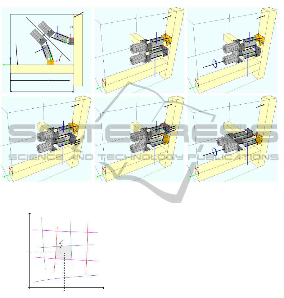
5.2 Phase 2: Concave Change of Plane
Once the beam b
2
has been reached, it can be climbed
to negotiate the structural node defined by the inter-
section of the three beams. The next objective is to
perform a concave transition between the faces f
1
and
f
2
. Note that at the end of the previous phase (Fig-
ure 6f), the Z axes of the frames attached to the two
feet point in the same direction. Hence, the postures
needed to change between these faces can be obtained
solving the PSIK problem defined in Section 4.
Figure 7a indicates the input parameters needed to
solve the PSIK problem: µ = 27.4 cm, ω = π/4 rad,
and j = B. Substituting these values and the geomet-
ric parameters of the robot into Eqs. (24)-(29) yields:
15.6 −2(16 −y
1B
−y
2B
)sinϕ
2B
2cos(ϕ
1B
−ϕ
2B
)
= 27.4 (32)
ϕ
2B
−π/4 = ϕ
1B
(33)
(4cosϕ
1B
−4)
2
+ (y
1B
+ 4 sin ϕ
1B
)
2
= r
2
1B
(34)
(4cosϕ
1B
−4)
2
+ (y
1B
−4 sin ϕ
1B
)
2
= l
2
1B
(35)
(4cosϕ
2B
−4)
2
+ (y
2B
+ 4 sin ϕ
2B
)
2
= r
2
2B
(36)
(4cosϕ
2B
−4)
2
+ (y
2B
−4 sin ϕ
2B
)
2
= l
2
2B
(37)
As discussed in Section 4, infinitely many solutions
exist since there are eight variables to be solved from
six equations. Next, we describe a way of choosing
a proper solution to this underconstrained problem.
First, Eq. (33) is used to eliminate ϕ
1B
from Eq. (32).
Then, ϕ
2B
is solved from the resulting equation:
ϕ
2B
= sin
−1
13.7
√
2 −7.8
y
1B
+ y
2B
−16
!
(38)
This solution can be substituted into Eqs. (33)-(37)
to express the joint coordinates
{
l
1B
,r
1B
,l
2B
,r
2B
}
in
terms of
{
y
1B
,y
2B
}
, which can be chosen so that
l
iB
,r
iB
∈ [19,25] (i = 1,2). Figure 8 represents the
curves of the (y
1B
,y
2B
) plane in which each joint co-
ordinate equals 19 or 25; any point inside the shaded
region R enclosed by these curves is a valid solu-
tion to the PSIK problem. For example, the solu-
tion y
1B
= y
2B
= 22 cm yields: r
1B
≈ 20.59536194,
l
1B
≈ 23.40761347, r
2B
≈ 23.65623783, and l
2B
≈
20.34961301, all in cm (these accurate values are
valid only for the simulation; in a real implementa-
tion we will have to deal with the finite precision of
the sensors). This solution is used to perform a transi-
tion between the faces f
1
and f
2
(see Figure 7a). After
performing this transition, the foot A is attached to the
beam b
2
, and the sequence of movements described in
Table 2 is used to complete this phase.
ICINCO2015-12thInternationalConferenceonInformaticsinControl,AutomationandRobotics
30
W
12 cm
4
0
c
m
5 cm
6 cm
leg A
leg B
leg A
leg B
r
1B
=l
1B
=19 cm
W
(a)
(b)
(c)
leg B
leg A
W
θ
A
= π rad
r
1B
=l
1B
=21 cm
leg B
leg A
W
leg B
leg A
r
1A
=l
1A
=19 cm
W
The feet A and B are
released and fixed resp.
θ
B
= π rad
W
leg B
leg A
(d)
(e)
(f)
b
1
b
1
b
1
b
1
b
1
b
1
b
2
b
2
b
2
b
2
b
2
b
2
Figure 6: Example trajectory where the robot moves along a beam of the structure.
Table 1: Sequence of movements in the first phase of the simulated trajectory.
Step Joint coordinates Description of the movements in each step
1 r
1B
= l
1B
= 19 cm Retract the actuators connected to the foot B to lift it (Figure 6b).
2 θ
A
= π rad Rotate the robot about the leg A (Figure 6c).
3 r
1B
= l
1B
= 21 cm
Extend the actuators connected to the foot B until it touches the beam b
1
(Figure 6d).
4 r
1A
= l
1A
= 19 cm
Attach the foot B to the face f
1
.
Release and lift the foot A retracting the actuators connected to it (Figure 6e).
5 θ
B
= π rad Rotate the robot about the leg B (Figure 6f).
Table 2: Sequence of movements in the second phase of the simulated trajectory.
Step Joint coordinates Description of the movements in each step
1
l
iA
= r
iA
= 21 cm
l
2B
= r
2B
= 21 cm
l
1B
= r
1B
= 19 cm
Lift the foot B and place both legs perpendicular to the face f
2
, leaving
some distance between the foot B and the face f
2
(Figure 7b).
2 θ
B
= π/2 rad Rotate the leg B about its own axis (Figure 7c).
3 r
1B
= l
1B
= 21 cm
Extend the actuators connected to the foot B until it touches the face f
2
(Figure 7d).
4 r
1A
= l
1A
= 19 cm
Attach the foot B to the face f
2
.
Release and lift the foot A retracting the actuators connected to it (Figure 7e).
5 θ
B
= π rad Rotate the robot about the leg B (Figure 7f).
KinematicAnalysisandSimulationofaHybridBipedClimbingRobot
31
(e)
(b)
leg B
W
88 cm
5 cm
µ
ω
leg A
55.6 cm
f
2
f
1
W
leg A
leg B
f
2
W
f
2
leg A
leg B
π/2
W
f
2
leg A
leg B
W
f
2
leg A
leg B
r
1B
=l
1B
=21 cm
r
1A
=l
1A
=19 cm
leg A
leg B
f
2
W
π/2
(a)
(
c
)
(d
)
(f
)
b
1
b
1
b
1
b
1
b
1
b
1
b
2
b
2
b
2
b
2
b
2
b
2
Figure 7: A trajectory that includes a concave transition between different planes.
r
1B
= 19
r
1B
= 25
l
1B
= 19
l
1B
= 25
r
2B
= 19
r
2B
= 25
l
2B
= 25
l
2B
= 19
15
30
15
30
R
y
1B
(cm)
y
2B
(cm)
22
22
Figure 8: Region of valid solutions to the PSIK problem.
5.3 Phase 3: Convex Change of Plane
At the end of phase 2, the Z axes of the frames at-
tached to the feet are parallel to the beam b
2
and
point in the same direction. Hence, the PSIK prob-
lem can be solved to determine the joint coordinates
that permit performing a convex transition from the
face f
2
to the face f
3
(the face f
3
is defined in Fig-
ure 9). Substituting µ = 11 cm, ω = 3π/4 rad, and
j = B in Eqs. (24)-(29), and following the procedure
detailed in Section 5.2, we can obtain the region of
the (y
1B
,y
2B
) plane where l
iB
,r
iB
∈ [19,25] cm (i =
1,2). It can be checked that the solution adopted
in the previous section (y
1B
= y
2B
= 22 cm) is also
valid here, obtaining in this case: r
1B
≈24.85374622,
l
1B
≈ 19.20940403, r
2B
≈ 21.99688208, and l
2B
≈
22.00311791 (all in cm). For these values of the joint
coordinates, the robot can perform a transition be-
tween the faces f
2
and f
3
(see Figure 9a). After that,
the foot A can be attached to the face f
3
.
After attaching the foot A to the face f
3
, the se-
quence of movements described in Table 3 is exe-
cuted. After executing this sequence, solving exactly
the same PSIK problem as in Section 5.2 permits the
foot A of the robot to be attached to the face f
4
of the
beam b
3
, which completes the trajectory.
6 CONCLUSIONS
This paper has presented the kinematic analysis of
a novel biped climbing robot with a hybrid serial-
parallel architecture. The forward kinematic problem
was solved, obtaining the relative position and orien-
tation between the feet in terms of the joint coordi-
ICINCO2015-12thInternationalConferenceonInformaticsinControl,AutomationandRobotics
32
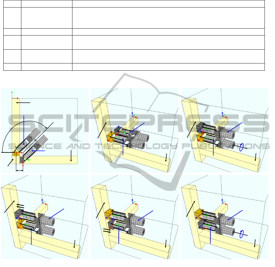
Table 3: Sequence of movements in the third phase of the simulated trajectory.
Step Joint coordinates Description of the movements in each step
1
l
iA
= r
iA
= 21 cm
l
2B
= r
2B
= 21 cm
l
1B
= r
1B
= 19 cm
Place both legs perpendicular to the face f
3
, leaving some distance between
the foot B and the face f
3
(Figure 9b).
2 θ
A
= 3π/2 rad Rotate the robot about the leg A (Figure 9c).
3 r
1B
= l
1B
= 21 cm
Extend the actuators connected to the foot B until it touches the face f
3
(Figure 9d).
4 r
1A
= l
1A
= 19 cm
Attach the foot B to the face f
3
.
Release and lift the foot A retracting the actuators connected to it (Figure 9e).
5 θ
A
= π rad Rotate the leg A about its own axis (Figure 9f).
(a)
(b) (c)
(d)
(e)
(f)
leg A
leg B
b
1
b
2
µ
b
3
ω
W
f
3
f
4
f
4
f
3
f
4
f
3
f
4
f
3
f
3
f
4
W
W
W
W
W
leg B
leg A
leg A
leg A
leg A
leg B
leg B
leg B
leg A
leg B
π/2
π/2
r
1B
=l
1B
=21 cm
r
1A
=l
1A
=19 cm
Figure 9: A trajectory that includes a convex transition between different planes.
nates. The inverse problem is more difficult due to the
redundancy of the robot. Hence, a simplified inverse
problem was analyzed. It was shown that the simpli-
fied problem is sufficient to perform some important
trajectories which are necessary to explore 3-D struc-
tures. This was shown using a tool that simulates the
kinematics of the robot and demonstrates its ability to
explore 3-D trusses.
To exploit all the possibilities offered by the
proposed kinematic architecture, the general inverse
kinematic problem of the robot will be solved in the
future. Other problems that will need to be addressed
include the determination of the workspace (positions
and orientations that are attainable from a given at-
tachment point), the dynamic modeling of the robot,
and the planning of trajectories avoiding collisions.
Also, the performance of the robot will be studied
in more complex structures (with beams having ar-
bitrary orientation, not just orthogonal frames), and a
real prototype of the robot is currently being devel-
oped to test it in a real structure.
KinematicAnalysisandSimulationofaHybridBipedClimbingRobot
33

ACKNOWLEDGEMENTS
This work was supported by the Spanish Government
through the Ministerio de Educaci
´
on, Cultura y De-
porte under a FPU grant (Ref: FPU13/00413) and
through the Ministerio de Econom
´
ıa y Competitivi-
dad under Project DPI2013-41557-P.
REFERENCES
Aracil, R., Saltaren, R. J., and Reinoso, O. (2006). A
climbing parallel robot: a robot to climb along tubular
and metallic structures. IEEE Robotics & Automation
Magazine, 13(1):16–22.
Baghani, A., Ahmadabadi, M. N., and Harati, A. (2005).
Kinematics Modeling of a Wheel-Based Pole Climb-
ing Robot (UT-PCR). In Proceedings of the 2005
IEEE International Conference on Robotics and Au-
tomation, pages 2099–2104.
Bajd, T., Mihelj, M., and Munih, M. (2013). Introduction
to Robotics. Springer Netherlands.
Balaguer, C., Gim
´
enez, A., Pastor, J. M., Padr
´
on, V. M.,
and Abderrahim, M. (2000). A climbing autonomous
robot for inspection applications in 3D complex envi-
ronments. Robotica, 18(3):287–297.
Figliolini, G., Rea, P., and Conte, M. (2010). Mechan-
ical Design of a Novel Biped Climbing and Walk-
ing Robot. In Parenti Castelli, V. and Schiehlen, W.,
editors, ROMANSY 18 Robot Design, Dynamics and
Control, volume 524 of CISM International Centre
for Mechanical Sciences, pages 199–206. Springer Vi-
enna.
Guan, Y., Jiang, L., Zhu, H., Zhou, X., Cai, C., Wu, W.,
Li, Z., Zhang, H., and Zhang, X. (2011). Climbot: A
modular bio-inspired biped climbing robot. In Pro-
ceedings of the 2011 IEEE/RSJ International Confer-
ence on Intelligent Robots and Systems, pages 1473–
1478.
Kong, X. and Gosselin, C. M. (2002). Generation and For-
ward Displacement Analysis of RPR-PR-RPR Ana-
lytic Planar Parallel Manipulators. ASME J. Mech.
Design, 124(2):294–300.
Mampel, J., Gerlach, K., Schilling, C., and Witte, H. (2009).
A modular robot climbing on pipe-like structures. In
Proceedings of the 4th International Conference on
Autonomous Robots and Agents, pages 87–91.
Schmidt, D. and Berns, K. (2013). Climbing robots for
maintenance and inspections of vertical structures - A
survey of design aspects and technologies. Robotics
and Autonomous Systems, 61(12):1288–1305.
Shvalb, N., Moshe, B. B., and Medina, O. (2013). A real-
time motion planning algorithm for a hyper-redundant
set of mechanisms. Robotica, 31(8):1327–1335.
Tavakoli, M., Marques, L., and De Almeida, A. T. (2011).
3DCLIMBER: Climbing and manipulation over 3D
structures. Mechatronics, 21(1):48–62.
Tavakoli, M., Viegas, C., Marques, L., Norberto Pires, J.,
and De Almeida, A. T. (2013). OmniClimber-II: An
omnidirectional climbing robot with high maneuver-
ability and flexibility to adapt to non-flat surfaces. In
Proceedings of the 2013 IEEE International Confer-
ence on Robotics and Automation, pages 1349–1354.
Tavakoli, M., Zakerzadeh, M. R., Vossoughi, G. R., and
Bagheri, S. (2005). A hybrid pole climbing and ma-
nipulating robot with minimum DOFs for construction
and service applications. Industrial Robot: An Inter-
national Journal, 32(2):171–178.
Yoon, Y. and Rus, D. (2007). Shady3D: A Robot that
Climbs 3D Trusses. In Proceedings of the 2007 IEEE
International Conference on Robotics and Automa-
tion, pages 4071–4076.
ICINCO2015-12thInternationalConferenceonInformaticsinControl,AutomationandRobotics
34
