
Inferential Active Disturbance Rejection Control of a Distillation
Column using Dynamic Principal Component Regression Models
Fahad Al Kalbani and Jie Zhang
School of Chemical Engineering and Advanced Materials, Newcastle University, Newcastle upon Tyne, NE1 7RU, U.K.
Keywords: Distillation Column, Composition Control, Inferential Control, Active Disturbance Rejection Control,
Principal Component Regression, Estimator.
Abstract: This paper presents a multivariable inferential active disturbance rejection control (ADRC) method for
product composition control in distillation columns. The proposed control strategy integrates ADRC with
inferential feedback control. In order to overcome long time delay of gas chromatography in measuring
product compositions, static and dynamic estimators for product compositions have been developed. The
top and bottom product compositions are estimated using multiple tray temperatures. In order to overcome
the colinearity issue in tray temperatures, principal component regression is used to build the estimator. The
proposed technique is applied to a simulated methanol-water separation column. It is shown that the
proposed control strategy gives good setpoint tracking and disturbance rejection control performance.
1 INTRODUCTION
Distillation is the most common and important
operation for purification and separation in industry.
According to Humphrey (1995) the United States
has around 40,000 distillation columns in operation
that handle more than 90% of purification and
separation processes. The capital investment for
these distillation systems is estimated to be around 8
billion US dollars. Referring to the data by Mix et al.
(1978), Soave and Feliu (2002) state that distillation
columns accounts approximately 3% of the total
world energy consumption which is equivalent to
about 2.87×10
18
J of energy per year. Unfortunately,
this enormous amount of energy is consumed in
providing heat to convert liquid to vapour and
condense the vapour back to the liquid at the
condenser.
With the growing environmental concern and
rising energy awareness, there is a need to reduce
the energy consumption in manufacturing industries.
Reducing the energy consumption of distillation
systems can be very effective in product cost
reduction because distillation can produce more than
50% of both capital and plant operating costs in a
typical chemical plant which can have a significant
impact on the overall plant profitability (Kiss and
Bildea, 2011)
. Therefore, extensive studies have
been carried out in recent years through the overall
system integration and new distillation design with
high energy efficiency. A suitable integration of
distillation columns with the total process leads to
substantial energy savings but the scope for this is
usually limited (Linnhoff, 1988). Therefore,
synthesis and design of new energy efficient
distillation systems and development of advanced
distillation control systems are both significant to
improve distillation technologies. As a result,
advanced and efficient control techniques are
required to reduce the energy consumption and to
meet the product compositions specifications. Strong
loop interactions exist between composition loops
that make distillation product composition control a
difficult task. Likewise, composition analyzers
usually introduce long time delay which affects the
achievable control performance.
In order to address these issues in distillation
column control, this paper presents an inferential
active disturbance rejection control (ADRC) method
which integrates ADRC with inferential control.
Multiple tray temperatures are used to estimate the
top and bottom product compositions. Since tray
temperatures are typically highly correlated,
multiple linear regressions would in this case not be
effective due to ill conditioning of the regression
data matrix. In order to overcome the colinearity
issue among tray temperatures, principal component
regression (PCR) is used to build the estimator
358
Al Kalbani F. and Zhang J..
Inferential Active Disturbance Rejection Control of a Distillation Column using Dynamic Principal Component Regression Models.
DOI: 10.5220/0005516703580364
In Proceedings of the 12th International Conference on Informatics in Control, Automation and Robotics (ICINCO-2015), pages 358-364
ISBN: 978-989-758-122-9
Copyright
c
2015 SCITEPRESS (Science and Technology Publications, Lda.)
models. Both static and dynamic PCR models are
developed. In dynamic PCR models, tray
temperature measurements at the current and past
sampling times are used as model inputs in order to
account for dynamic relationship between tray
temperatures and product compositions. To the
authors’ knowledge, the integration of ADRC and
dynamic inferential control has not been reported in
the literature.
This paper is organised in five sections. Section
2 presents an overview of ADRC and inferential
control. Section 3 presents the development of static
and dynamic estimator using PCR. The inferential
feedback control of distillation compositions based
on these software sensors is represented in Section 4.
Finally, the last section draws some concluding
remarks.
2 OVERVIEW OF ADRC AND
INFERENTIAL CONTROL
Disturbances and uncertainties are the main issues in
control system synthesis especially in engineering
applications. Dealing with disturbances and
uncertainties has attracted the attention of engineers
and scientists. There have been many control
methods suggested for dealing with uncertainties
such as adaptive control, robust control, variable
structure control, intelligent control, etc. However,
due to their dependence and complexity on advanced
analytical methodologies, these methods have
certain limitations in engineering applications.
PID control is still widely used in process control
because of its simplicity and robustness. The main
limitations of PID control are the error computation,
noise degradation due to the derivative control,
oversimplification and the loss of performance in the
control law in the form of linear weighted sum and
complication associated to the integral control.
2.1 Overview of ADRC
ADRC, derived the essence from PID control and
observer, was pioneered over ten years ago by
Jingqing Han (Han, 2009). The basic principle of
ADRC is that it uses the extended state observer
(ESO) to estimate the existing total disturbances,
and cancel it or remove it from the system. The main
advantage of ADRC is the disturbance rejection
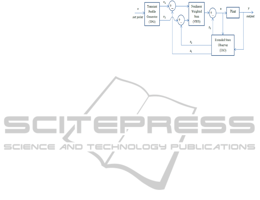
(Gao et al, 2011). Fig. 1 shows the structure of
ADRC, which consists of three main components:
transient profile generator (TPG), non-linear
weighted sum (NWS), and ESO.
Figure 1: Structure of ADRC.
A. Transient Profile Generator
The control signal with TPG can rapidly track the
setpoint signal without overshoot with strong
adaptability and robustness (Wang and Miao, 2010).
TPG can smooth out sudden changes in setpoints.
B. Non-linear Weighted Sum of Control Errors
Over-simplification of PID control law is the major
limitation of the conventional PID controller that
consists of present, predictive and accumulative
errors. This over-simplification ignores other
complex parameters that can make the PID control
performance more robust to the error signal. As a
result, Han (2009) presented an alternative non-
linear function which depends on the magnitude of
error signal to produce the control signal.
C. Extended State Observer
The main idea of ESO is to online estimate the
variables that are usually inapproachable
instrumentation-wise such as internal non-linear
dynamics, external disturbance and model errors.
Then, the undesired disturbances are then effectively
compensated in the control effort. ADRC can
successfully drive the controlled output signal to its
required value if the ESO has a precise estimation
for the internal non-linear dynamics, external
disturbances and model error of the plant (Xia et al,
2007).
2.2 Overview of Inferential Control
In the product composition control in distillation
columns, it is really challenging to get reliable and
accurate product composition measurements without
long time delay in the sampling and analysis
process. Numerous composition analysers such as
gas chromatography regularly introduce significant
time delays. The overall time delay in composition
measurements normally between 10 to 20 minutes
(Mejdell and Skogested, 1991). Such amount of time
delay substantially reduces the achievable
performance of composition controllers. Moreover,
InferentialActiveDisturbanceRejectionControlofaDistillationColumnusingDynamicPrincipalComponentRegression
Models
359
the reliability of the composition analysers is usually
quit low and incurs high maintenance cost.
Therefore, in distillation composition control, it is a
usual practice to indirectly control product
compositions by controlling tray temperatures or
utilize the secondary tray temperature measurements
to estimate and control the product compositions.
Compared with composition measurements,
temperature measurements are more economic,
reliable and virtually without any measurements
time delays.
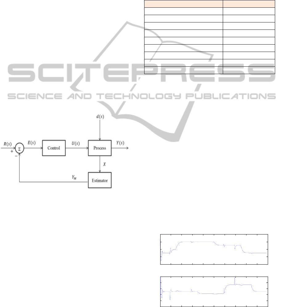
The estimator based inferential feedback control
structure for product composition control in a binary
distillation column is depicted in Fig. 2. The
estimated variable is used instead of the measured
variable to overcome the long measurement delay.
The manipulated variables for composition control
are the reflux rate (L) and steam flow rate to the
reboiler (V). A sample of variable X (tray
temperature) is taken continuously and sent it to
estimator to estimate the output Y(s) (product
composition) and generate signal Y
M
as a feedback
signal. The feedback controller can be any such as a
multi-loop controller or a multivariable controller.
Figure 2: Inferential feedback control.
3 PCR MODEL BASED
SOFTWARE SENSORS
The distillation columns presented in this paper is
comprehensive non-linear simulation of a methanol-
water separation column. A non-linear tray by tray
mechanistic model has been developed using mass
and energy balances. The following assumptions are
made: constant liquid holdup, negligible vapour
holdup and perfect mixing in each stage. The
nominal operation data for this specific column are
given in Table 1.
The nominal operating point considered in this
study is the top composition at 93% and the bottom
composition at 7%. To generate data for building
PCR inferential estimation models, series of random
disturbances were added. Fig. 3 shows the top and
bottom product compositions in the generated data.
Fig. 4 shows the corresponding tray temperature
data. It can be realized that correlation exists among
tray temperature measurements.
Table 1: Nominal distillation column operation data.
Variables Nominal values
Top concentration (y
1
) 93 % methanol
Bottom concentration (y
2
) 7 % methanol
Top product rate (D) 9.13 g/s
Bottom product rate (B) 9.1 g/s
Reflux flow rate (u
1
) 10.108 g/s
Steam flow rate (u
2
) 13.814 g/s
Feed concentration (d
1
) 50.12 %
Feed flow rate (d
2
) 18.23 g/s
No. of trays 10
3.1 Static PCR Model
In the static model, the product compositions at time
t are estimated from tray temperatures at time t. The
model can be defined in the following form:
)()()()(
10102211
tTtTtTty
θ
θ
θ
+++=
(1)
where y represents the product compositions, T
1
to T
10
denote the tray temperatures from tray 1 to
tray 10 respectively, θ
1
to θ
10
are model parameters
corresponding to tray temperatures, and t indicates
the discrete time.
The data were scaled to zero mean and unit
variance before model building to allow data with
different ranges to be used within the same model.
Then, the data is divided into training data set
(samples 1 to 1189) and the testing data set (samples
1190 to 1982). PCR models with different numbers
of principal components were developed on the
training data and tested on the testing data.
0 200 400 600 800 1000 1200 1400 1600 1800 2000
90
92
94
96
98
time(minute)
Top comp y
D
. (%)
0 200 400 600 800 1000 1200 1400 1600 1800 2000
2
4
6
8
10
12
time(minute)
Bot comp y
B
. (%)
Figure 3: Top and Bottom product compositions.
ICINCO2015-12thInternationalConferenceonInformaticsinControl,AutomationandRobotics
360
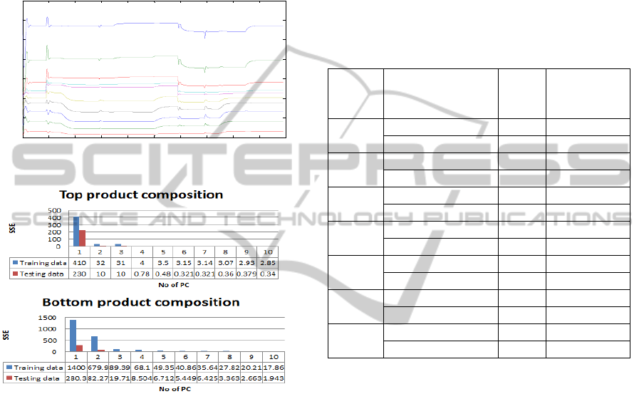
Fig. 5 represents the sum of squared errors (SSE) of
PCR models with different number of principal
components on the training and testing data. The
number of principal components is determined based
on the minimum value of SSE on the testing data.
The PCR model with the lowest SSE on the testing
data is considered as having the appropriate number
of principal components.
0 200 400 600 800 1000 1200 1400 1600 1800 2000
65
70
75
80
85
90
95
100
time(minute)
Tray temperature(C)
Figure 4: Tray temperatures.
Figure 5: SSE of different PCR models.
It can be seen from Fig. 5 that 6 principal
components offers the best performance for the top
composition on the testing data and 10 principal
components give the best performance for the
bottom composition. Hence, the suitable numbers of
principal components for the top and bottom
compositions were specified as 6 and 10
respectively. The SSE on the testing data is 0.34 for
the top composition and 1.943 for the bottom
composition.
3.2 Dynamic PCR Model
The accuracy of inferential estimation could be
further enhanced and improved if a dynamic PCR
module is developed. Seven dynamic models with
different orders were developed. As an example, the
first order dynamic PCR model is of the following
form:
)1()()1(
)()1()()(
102.10101.1022.2
21.222.111.1
−++−
++−+=
tTtTtT
tTtTtTty
θθθ
θ
θ
θ
(2)
Data partition and data scaling are the same as in
building the static PCR model. By taking the least
SSE, the appropriate numbers of principal
components can be determined. Table 2 presents the
numbers of principal components and the SSE on
the testing data of these dynamic PCR models.
Table 2: Number of principal components and SSE on
testing data of different dynamic PCR models.
Model
orders
SSE
No. of
principal
components
1
Top composition 0.662 11
Bot composition 13.04 11
2
Top composition 0.361 14
Bot composition 9.958 7
3
Top composition 0.045 32
Bot composition 2.970 7
4
Top composition 0.140 50
Bot composition 2.542 7
5
Top composition 0.122 17
Bot composition 1.323 7
6
Top composition 0.145 42
Bot composition 4.722 8
7
Top composition 0.141 54
Bot composition 3.958 8
It can be realized that the dynamic PCR models
substantially improve the estimation accuracy over
the static PCR especially the third order, fourth order
and fifth order models. All these three models has
been compared and discussed. The difference
between these three models is not significant. Thus
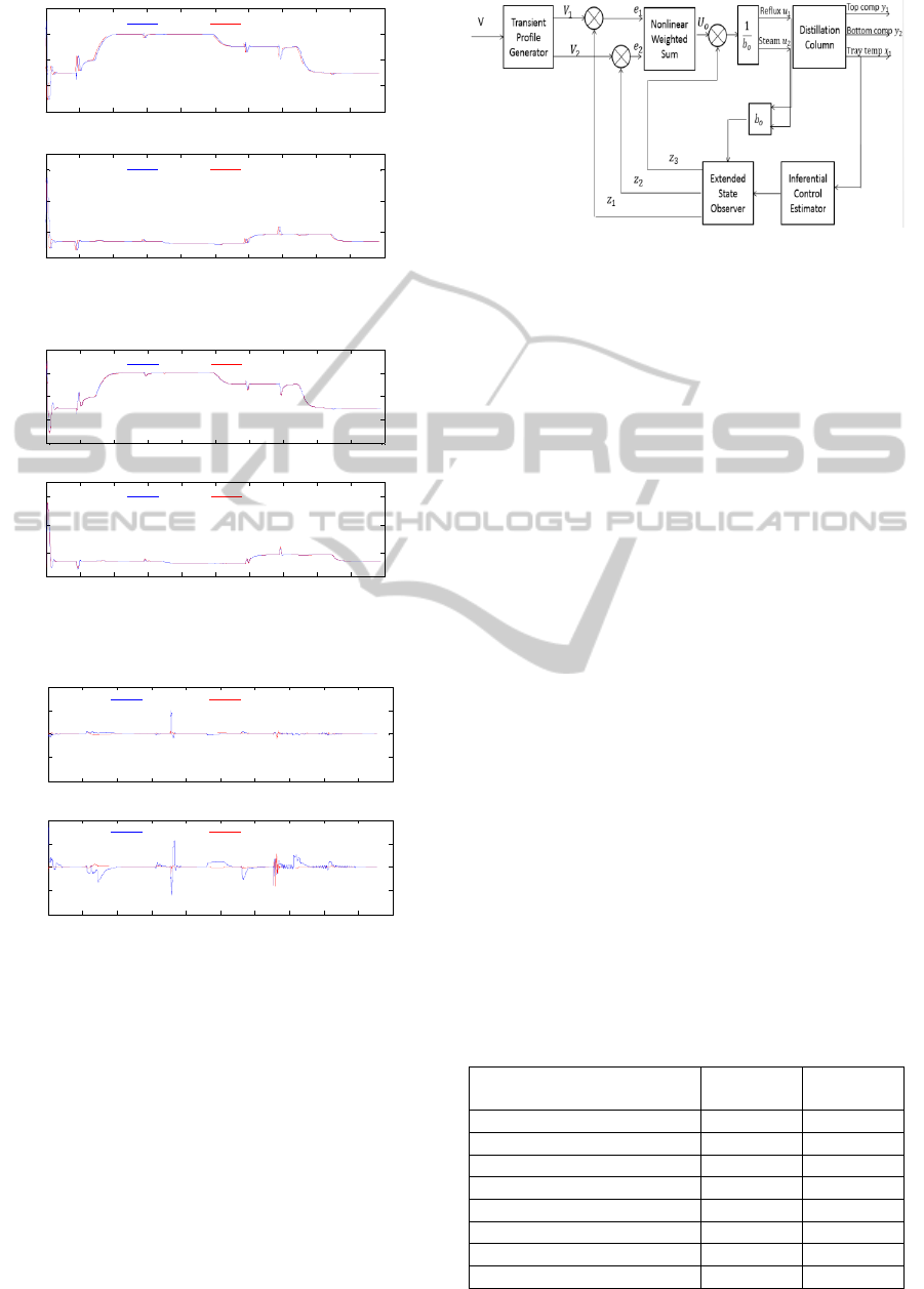
the fifth order dynamic PCR model is used. Fig. 6
and Fig. 7 show, respectively, the predictions of the
static PCR model and the 5
th
order dynamic PCR
model. In these figures, the solid lines represent the
actual measured compositions response while the
dashed lines represent the corresponding model
estimations predictions. Fig. 8 shows the estimation
errors. It can be realized that the 5
th
order dynamic
PCR model gives better performance and more
accurate predictions or estimation than the static
model.
It can be seen from Table 2 that the dynamic
PCR models quite significantly enhance the
estimation accuracy over the static PCR model,
especially the fourth order and fifth order models.
The fifth order dynamic PCR model is given in the
appendix.
InferentialActiveDisturbanceRejectionControlofaDistillationColumnusingDynamicPrincipalComponentRegression
Models
361
0 200 400 600 800 1000 1200 1400 1600 1800 2000
90
92
94
96
98
time(minute)
Top comp y
D
. (%)
Actual y
D
Estimated y
D
0 200 400 600 800 1000 1200 1400 1600 1800 2000
10
20
30
time(minute)
Bot comp y
B
. (%)
Actual y
B
Estimated y
B
Figure 6: Model predictions of the static PCR model.
0 200 400 600 800 1000 1200 1400 1600 1800 2000
90
92
94
96
98
time(minute)
Top comp y
D
. (%)
Actual y
D
Estimated y
D
0 200 400 600 800 1000 1200 1400 1600 1800 2000
10
20
30
time(minute)
Bot comp y
B
. (%)
Actual y
B
Estimated y
B
Figure 7: Model predictions the 5
th
order dynamic PCR
model.
0 200 400 600 800 1000 1200 1400 1600 1800 2000
-1
-0.5
0
0.5
1
time (minutes)
Error signal -Top comp y
D
.
static model
5th dynamic model
0 200 400 600 800 1000 1200 1400 1600 1800 2000
-0.4
-0.2
0
0.2
0.4
time (time)
Error si gnal-Bot comp y
B
static model
5th dynamic model
Figure 8: Error signal between the actual and estimated
signal.
4 INFERENTIAL ADRC OF
DISTILLATION
COMPOSITION BASED ON
PCR MODELS
The ADRC scheme and inferential control are
integrated together to control the top and bottom
compositions in the distillation column. The
integrated inferential ADRC is shown in Fig. 9.
Figure 9: ADRC integrated with the inferential control.
Eight inferential feedback control schemes with
eight different software sensors (static and the first
to the seventh order dynamic PCR models) were
designed and developed.
To investigate the performance of both static and
dynamic order models, the following disturbance
were added to the simulated distillation column. The
feed rate was increased by 15% at the 200
th
minutes
and the 1200
th
minutes, the feed composition was
increased by 15% at the 1400
th
minutes.
Furthermore, series setpoints changes are applied to
both top and bottom product compositions. Table 3
shows the SSE (the difference between actual and
estimated) of different schemes under the distur-
bances. It can be seen that the dynamic PCR
schemes gives better performance than static PCR
model especially the 3
rd
and 5
th
order dynamic PCR
model based schemes.
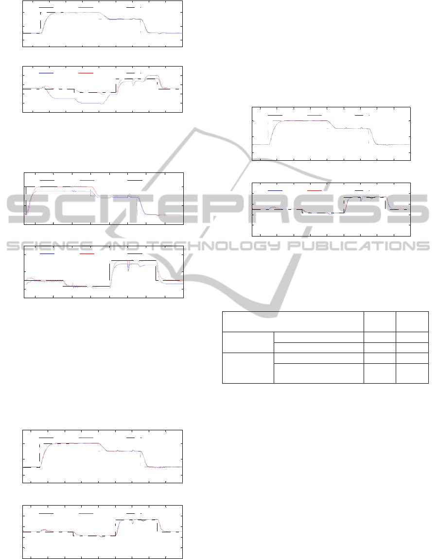
Fig. 10 and Fig. 11 demonstrate respectively the
responses of static inferential ADRC scheme and
dynamic inferential ADRC across a wide range of
setpoint changes, feed composition and feed flow
rate disturbances. The setpoint signal was smoothed
by TPG. It can be seen that both compositions are
well controlled and dynamic inferential ADRC gives
better performance than the static inferential ADRC
despite of large static control errors exist for the
bottom product composition. This static control error
generated due to the PCR model errors, which can
be large when operating condition changes such as
setpoint changes and/or disturbance changes.
Table 3: SSE of different control schemes.
Control schemes
SSE in Top
comp
SSE in
Bottom comp
Static PCR module 1.6889 1.8309
1
st
order dynamic PCR model 0.2152 4.7203
2
n
d
order dynamic PCR model 0.8406 11.0903
3
r
d
order dynamic PCR model 0.2118 0.7080
4
th
order dynamic PCR model 2.6854 1.5137
5
th
order dynamic PCR model 0.1856 0.1551
6
th
order dynamic PCR model 1.2277 1.3307
7
th
order dynamic PCR model 0.4868 0.2600
ICINCO2015-12thInternationalConferenceonInformaticsinControl,AutomationandRobotics
362
200 400 600 800 1000 1200 1400 1600 1800 2000
92
94
96
time (minutes)
Top comp
y
D
. (%
)
Actual y
D
Estimated y
D
Setpoint y
D
200 400 600 800 1000 1200 1400 1600 1800 2000
2
4
6
8
10
12
time
(
minute
)
Bot comp
y
B
. (%
)
Actual y
B
Estimated y
B
Setpoint y
D
Figure 10: Responses of actual and estimated product
compositions of static inferential ADRC (without mean
updating).
200 400 600 800 1000 1200 1400 1600 1800
92
94
96
time (minutes)
Top comp y
D
. (%)
Actual y
D
Estimated y
D
Setpoint y
D
200 400 600 800 1000 1200 1400 1600 1800
6
8
10
time (time)
Bot comp y
B
. (%)
Actual y
B
Estimated y
B
Setpoint y
D
Figure 11: Responses of actual and estimated product
compositions of 5
th
dynamic inferential ADRC (without
mean updating).
To overcome the static control off-sets issues due to
the continuous changes in process operating
conditions, mean updating strategy proposed by
Zhang (2006) is implemented here to eliminate
control off-set and static estimation. The main idea
200 400 600 800 1000 1200 1400 1600 1800 2000
92
94
96
time (minutes)
Top comp y
D
. (%)
Actual y
D
Estimated y
D
Setpoint y
D
200 400 600 800 1000 1200 1400 1600 1800 2000
2
4
6
8
10
12
time (minute)
Bot comp y
B
. (%)
Actual y
B
Estimated y
B
Setpoint y
D
Figure 12: Responses of actual and estimated product
compositions of static inferential ADRC (with mean
updating).
of mean updating strategy is that when a new steady
state is detected, the process variable means are
updated. Hence model predictions will be updated. It
should be noted here that only occasional product
composition measurements are required. Fig. 12 and
Fig. 13 indicate the control performance with mean
updating technique. It can be shown from these
figures that, by using the mean updating technique,
the static control offsets are eliminated.
200 400 600 800 1000 1200 1400 1600 1800 2000
92
94
96
time (minutes)
Top comp y
D
. (%)
Actual y
D
Estimated y
D
Setpoint y
D
200 400 600 800 1000 1200 1400 1600 1800 2000
2
4
6
8
10
12
time (minute)
Bot comp y
B
. (%)
Actual y
B
Estimated y
B
Setpoint y
D
Figure 13: Responses of actual and estimated product
compositions of 5
th
dynamic inferential ADRC (with mean
updating).
Table 4: SSE of different control schemes.
Control schemes
Top
Comp
Bottom
Comp
Static PCR
model
Without mean updating 54542 6946.9
With mean updating 1.6889 1.8309
5
th
order
dynamic PCR
model
Without mean updating 165.52 219.59
With mean updating 0.1856 0.1551
It can be seen from above figures that the resulting
control off-sets and steady state model estimation
bias have been eliminated through the mean
updating technique. Moreover, it can be noticed
from Table 4 that the dynamic PCR model has much
smaller estimation off-sets than the static PCR
model when the operating condition changed. This
leads to a result that the dynamic PCR model is
more robust than the static PCR model to process
operating condition variations.
5 CONCLUSIONS
Static and dynamic inferential ADRC control
schemes are proposed for product composition
control in distillation columns. Inferential estimation
models for product compositions are developed from
process operational data using PCR. The estimated
InferentialActiveDisturbanceRejectionControlofaDistillationColumnusingDynamicPrincipalComponentRegression
Models
363

product compositions are used as the controlled
variables in the ADRC controller. Mean updating
technique is used to eliminate the steady state model
estimation bias and the resulting control off-sets.
The proposed control method is applied to a
simulated methanol-water separation column.
Simulation results indicate the effectiveness and
success of the proposed dynamic inferential ADRC
control method over the static inferential ADRC
control method.
REFERENCES
Gao, Z., Hu, S. H., Jiang, F.J. (2001), A novel motion
control design approach based on active disturbance
rejection, Proceedings of the 40th IEEE Conference on
Decision and Control, 1-5, 4877-4882.
Han, J. (2009). From PID to active disturbance rejection
control. IEEE Trans. Ind. Electronics, 56(3), 900-906.
Humphrey, J. (1995) Separation processes: playing a
critical role. Chemical Engineering Progress, 91(10),
pp. 43-54.
KISS, A. A. and BILDEA, C. S. (2011). A control
perspective on process intensification in dividing-wall
columns. Chemical Engineering and Processing, 50,
281-292.
Linnhoff, B. (1988). Distillation design. Chemical and
Engineering Results Design, pp 1 - 30.
Mejdell, T. and Skogestad, S. (1991). Estimation of
distillation compositions from multiple temperature
measurements using partial-least-squares regression.
Industrial & Engineering Chemistry Research, 30(12),
pp.2543-2555.
Mix, T., Dweck, J.S., Weinberg, M., Armstrong, R.C.
(1978) Energy conservation in distillation. Chemical
Engineering Progress, 74(4), 49-55.
Soave, G. and Feliu, J. (2002) Saving energy in distillation
towers by feed splitting. Applied Thermal
Engineering, 22(8), pp. 889-896.
Xia, Y., Shi, P., Liu, G. P., Rees, D., Han, J. (2007).
Active disturbance rejection control for uncertain
multivariable systems with time-delay. IET Control
Theory and Applications, 1(1), 75-81.
Wang, Y. and Miao, J. (2010) Electrode regulator system
for ore smelting electric arc furnace based on active
disturbance rejection control technology. Proceedings
of the 2010 IEEE International Conference on
Advanced Computer Control, 109-113.
Zhang, J. (2006). Offset-Free inferential feedback control
of distillation composition based on PCR and PLS
models, Chemical Engineering and Technology, 29(5),
560-566.
APPENDIX
Model parameters of the 5
th
order dynamic model
Table 5: Top composition parameters.
t t-1 t-2 t-3 t-4 t-5
T
1
-0.037 0.006 0.077 0.0914 0.0385 -0.151
T
2
0.0121 -0.039 -0.030 -0.061 0.031 -0.001
T
3
0.115 0.059 0.031 -0.021 -0.002 -0.030
T
4
0.0513 0.014 -0.003 -0.035 -0.009 -0.020
T
5
0.0464 -0.022 -0.021 -0.044 -0.052 -0.016
T
6
-0.083 -0.045 0.056 0.068 0.065 0.016
T
7
-0.138 -0.069 0.020 0.044 0.071 0.055
T
8
-0.171 -0.110 -0.042 -0.023 0.004 0.007
T
9
-0.175 -0.103 -0.015 0.013 0.068 0.100
T
10
-0.219 -0.146 -0.088 -0.071 -0.047 -0.017
Table 6: Bottom composition parameters.
t t-1 t-2 t-3 t-4 t-5
T
1
-0.569 -0.453 -0.307 -0.140 0.032 0.191
T
2
-0.122 -0.084 -0.037 0.0419 0.154 0.261
T
3
0.0559 0.052 0.0471 0.0596 0.0997 0.142
T
4
0.0191 -0.004 -0.041 -0.076 -0.093 -0.097
T
5
0.083 0.059 0.020 -0.033 -0.084 -0.122
T
6
0.113 0.065 0.016 -0.028 -0.005 -0.062
T
7
0.002 -0.027 -0.047 -0.053 -0.041 -0.015
T
8
0.032 0.014 0.004 0.007 0.026 0.055
T
9
-0.008 -0.033 -0.048 -0.048 -0.027 0.0079
T
10
0.017 0.001 -0.004 0.0026 0.028 0.0669
ICINCO2015-12thInternationalConferenceonInformaticsinControl,AutomationandRobotics
364
