
Computationally Efficient Multiphase Heuristics for Simulation-based
Optimization
Christoph Bodenstein, Thomas Dietrich and Armin Zimmermann
Systems & Software Engineering, Ilmenau University of Technology, P.O. Box 100 565, 98684 Ilmenau, Germany
Keywords:
SCPN, Petri Nets, Simulation, Optimization.
Abstract:
Stochastic colored Petri nets are an established model for the specification and quantitative evaluation of com-
plex systems. Automated design-space optimization for such models can help in the design phase to find good
variants and parameter settings. However, since only indirect heuristic optimization based on simulation is
usually possible, and the design space may be huge, the computational effort of such an algorithm is often
prohibitively high. This paper extends earlier work on accuracy-adaptive simulation to speed up the overall
optimization task. A local optimization heuristic in a “divide-and-conquer” approach is combined with vary-
ing simulation accuracy to save CPU time when the response surface contains local optima. An application
example is analyzed with our recently implemented software tool to validate the advantages of the approach.
1 INTRODUCTION
Stochastic Colored Petri nets (Zenie, 1985; Zimmer-
mann, 2007) are well-known for their rich modeling
and event-based simulation capabilities for complex
systems. A realistic simulation model can assist in
finding the right set of design parameter settings. To
find the optimal configuration, so-called optimization
by simulation (or indirect optimization) can be ap-
plied. This is a commonly used approach as found
in (Fu, 1994b; Carson and Maria, 1997; Fu, 1994a;
Biel et al., 2011; K
¨
unzli, 2006). The data flow of the
usual setup is depicted in Figure 1.
The design space for optimization is defined by
the number of parameters and their individual value
ranges. This design space can be very large or even in-
finite, and because each parameter set has to be eval-
uated with a simulation that may require several min-
utes of CPU time, the overall time for a full design
space scan is intractable. Heuristics such as simulated
annealing, hill climbing, genetic algorithms etc. are
solutions for this problem that exchange some result
accuracy for a significant speedup in many practical
examples.
Often not only one design-space optimization
heuristic exists that fits the whole solution process:
in the beginning, a rough global search for a promis-
ing region is beneficial, while the accuracy of the fi-
nal result can be improved by a fine-grained local
search at the end. Two-phased heuristics are there-
fore used (Schoen, 2002) and mix, for instance, simu-
lated annealing for the start with a hill-climbing local
search at the end.
However, despite this combination of heuristics
and the development of many specialized heuris-
tics, another idea (that may be combined with it) is
to also take into consideration the accuracy of the
model analysis. This uses explicitly the trade-off be-
tween solution accuracy and computational effort. A
first step is a two-phase approach for instance taken
in (Rodriguez et al., 2004; Zimmermann et al., 2001),
where the detailed stochastic Petri net models of man-
ufacturing systems are approximately and rapidly an-
alyzed during the first phase (based on performance
bounds), while a correct detailed simulation is done
finally.
In our current work we aim at extending this vari-
ant of the two-phase idea towards adaptively control-
ling the evaluation accuracy based on the result qual-
ity that the heuristic currently needs (Zimmermann
and Bodenstein, 2011). The contribution of this idea
is a tighter integration between the two modules of in-
Sim. Output
Parameter set
Optimization
heuristic
Simulation
Figure 1: Common black box optimization, see (Carson and
Maria, 1997).
95
Bodenstein C., Dietrich T. and Zimmermann A..
Computationally Efficient Multiphase Heuristics for Simulation-based Optimization.
DOI: 10.5220/0005518000950100
In Proceedings of the 5th International Conference on Simulation and Modeling Methodologies, Technologies and Applications (SIMULTECH-2015),
pages 95-100
ISBN: 978-989-758-120-5
Copyright
c
2015 SCITEPRESS (Science and Technology Publications, Lda.)
direct optimization and its use for algorithm speedup.
There are many ways to control the accuracy of eval-
uation — a first simple method is to adapt the dis-
cretization step of the design parameters (adapting
model detail granularity or refinement quality was
proposed for this in (Zimmermann and Bodenstein,
2011), but without an automated tool implementa-
tion).
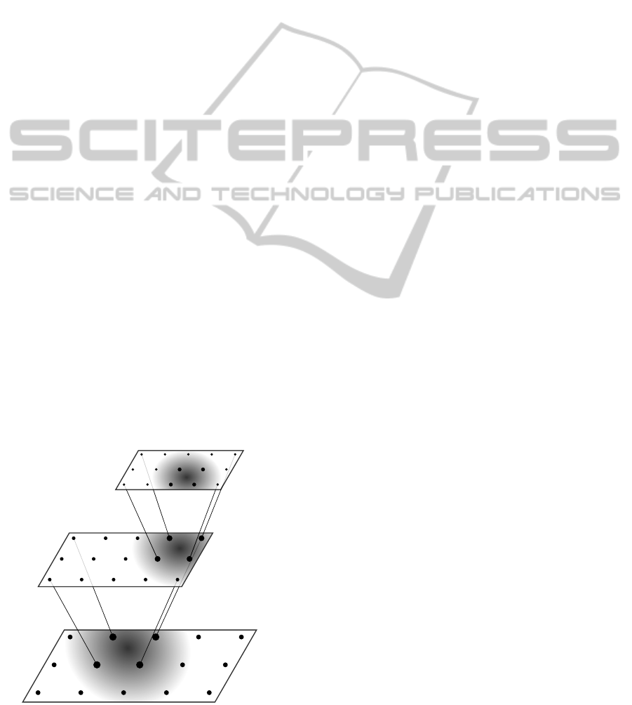
Figure 2 shows the principle of such a multi-phase
optimization heuristic. The same base heuristic is ap-
plied in every phase. The resolution of all parame-
ters (discretization step) is reduced at the beginning
of the algorithm. Thus the search will be faster and
concentrate on the best found regions in the following
phases, looking at them more closely with a smaller
step size. Only the final phase makes use of the orig-
inally defined parameter discretization. Obviously
there is the risk of not finding the global optimum
in such a method, depending on the relation between
step size and steepness of the optimized function.
First results of this approach for stochastic col-
ored Petri nets have been reported in (Boden-
stein and Zimmermann, 2015). The generic con-
trol algorithm has been implemented as an exten-
sion of our Petri net modeling and evaluation soft-
ware TimeNET (Zimmermann, 2012), a tool de-
scription of the optimization has been published re-
cently (Bodenstein and Zimmermann, 2014). It
allows to control optimization experiments in a
user-friendly way. The software package is avail-
able free of charge for non-commercial use at
http://www.tu-ilmenau.de/timenet.
In the presented paper, this approach is extended
to control not only the discretization of parameter
value ranges, but also the targeted accuracy of every
simulation run. The simulation accuracy is specified
Figure 2: Principle idea of a multi-phase heuristic.
in TimeNET by confidence interval size (by means of
a relative error, usually around 5% percent), and the
probability of the actual result to be within the con-
fidence interval (a quantile-like probability, typically
around 95%).
The simulation accuracy is initially set to a low
value and increases in a stepwise fashion until its
maximum value is reached in the final phase. By
doing so, most of the simulations are executed with
a low accuracy and significantly less CPU time con-
sumption, while a high accuracy is achieved in the
end.
As a result, optimizing a model utilizing a multi-
phase optimization heuristic should save CPU time
compared to the described one- or two-phase opti-
mization approaches, even if more simulation runs
may be necessary. The contribution of this paper
is the proposal of the described variant of accuracy-
adaptive optimization heuristic, its implementation in
a publicly available software tool, and application ex-
periments that demonstrate the speedup.
The paper first introduces a formula to approxi-
mate the CPU time depending on accuracy control pa-
rameters by analyzing the results of experiments done
with real SCPN simulations. Different configurations
of a multi-phase optimization heuristic are evaluated
afterwards.
As real simulation-based optimizations take a lot
of actual computation time, we decided to analyze the
proposed combined heuristic with analytical bench-
mark functions first. The selected combination con-
sists of functions with typical tripping hazards for
optimization algorithms and reflect typical hard de-
sign space problems. The reference benchmark func-
tions Matya, Sphere, Schwefel, and Ackley (Jamil
and Yang, 2013) were selected. Finally, the paper
presents results of several experiments showing typ-
ical dependencies between achievable speedup, result
accuracy, and optimal parameter set distance on one
hand and the number of accuracy-changing phases of
our algorithm. The results validate our hypothesis that
an adaptive control is advantageous compared to re-
stricting heuristics to only two phases.
2 RELATIONSHIP BETWEEN
ACCURACY AND CPU TIME OF
AN SCPN SIMULATION
Cost functions for SCPN simulations are defined by
a performance measure (Sanders and Meyer, 1991).
The optimization heuristic aims to minimize (or max-
imize) the result by varying parameter values. SCPNs
SIMULTECH2015-5thInternationalConferenceonSimulationandModelingMethodologies,Technologiesand
Applications
96
can be simulated in two different ways, which are also
supported by the tool TimeNET: The first is a tran-
sient analysis where the user defines the simulation
end time. The simulation is executed repeatedly and
the measurements are calculated at specific points in
simulation time. The simulation is stopped if all mea-
sures at all defined points in simulation time reached
their required accuracy.
The second type is a stationary simulation. A
model is simulated until all measures meet the prede-
fined accuracy constraints. The model must not have
dead states in this case.
The desired accuracy of an SCPN simulation is
specified by two parameters in the tool, namely, con-
fidence interval and maximum relative error. The
confidence interval is usually chosen between 85%
and 99%, which means that this amount of all mea-
sured values are estimated to be within a defined
range around the average (expected) value. The size
of this range is defined by the maximum relative error
(15% down to 1%). The three parameters confidence
interval, maximum relative error, and necessary CPU
time for one simulation run show characteristic de-
pendencies as depicted in Figure 3 (Bodenstein and
Zimmermann, 2015).
Conf.-Intervall(85-99)
Max Error(1-10)
CPU-Time
+
+
+
+
+
+
+
+
+
+
+
+
+++
+
+
+
+
+
+
+
+
+
+
+
+
+
+
+
+++++
+
+
+
+
+
+
+
+
+
+
+
+
+
+
+
+
+
+
+
+
+
+
+
+
+
+
+
+
+
+
+
+
+
+
+
+
++++
+
+
+++
+
+
+
+
+
+
+
+
+
+
+
+
+
+
+
+
+
+
+
+
+
+
+
++
+
+
+
+
++
+
+
+
+
+
+
+
+
+
+
+
+
+
+
+
+
+
+
+
+
+
+
+
+
+
+
+
+
+
+
+
+
+
+
+
+
+
+
+
500
1000
1500
Figure 3: Example relation for confidence interval / maxi-
mum relative error vs. CPU time.
For a later estimation of speedups for the model
optimization for which this correlation was measured,
the approximate formula 1 for the relation shown in
the figure has been fitted. Values cc and me represent
confidence interval and maximum relative error, re-
spectively. Both are normalized to values between 1
and 15.
CPUTime =
cc ∗ me
a
3
· b + c (1)
In our experiments, we determined values of a =
49.74, b = 23.91, c = 154.29, resulting in a cal-
culated CPU time between 110 and 2300 seconds.
This approximation combined with benchmark func-
tions allowed to analyze the benefits of a multi-phase-
heuristic in terms of CPU time consumption without
using real simulations first.
3 BENCHMARK FUNCTIONS
FOR HEURISTIC
OPTIMIZATION
As result functions of SCPN performance measures
can have very different shapes we chose four char-
acteristic benchmark functions to emulate the behav-
ior of real SCPN simulations according to parameter
variation.
Although there are many other functions we hope
to cover most SCPN relevant function shapes with the
chosen benchmark functions. They are characterized
as follows:
Sphere. A simple function which can be calculated
for any number of input variables. It is defined for
x
i
∈ [−5; 5] (Rajasekhar et al., 2011) and shown in
figure 4.
f (
−→
x ) =
D
∑
i=1
x
2
i
(2)
Matya. This function is only defined for two input
variables, but its shape is interesting as it has a
wide range of parameter values to result in near-
optimum output values. Therefore it is hard to
find the absolute optimum in definition space for
any optimization heuristic (Bodenstein and Zim-
mermann, 2015; Rajasekhar et al., 2011).
f (x, y) = 0.26(x
2
+ y
2
) − 0.48xy (3)
Figure 4: Sphere and Matya benchmark functions.
Ackley. A very popular function as it is defined for
any number of input variables and because of its
symmetric shape and several local optima (shown
in Figure 5). This function is hard to tackle with
common optimization heuristics (Rajasekhar
et al., 2011).
ComputationallyEfficientMultiphaseHeuristicsforSimulation-basedOptimization
97
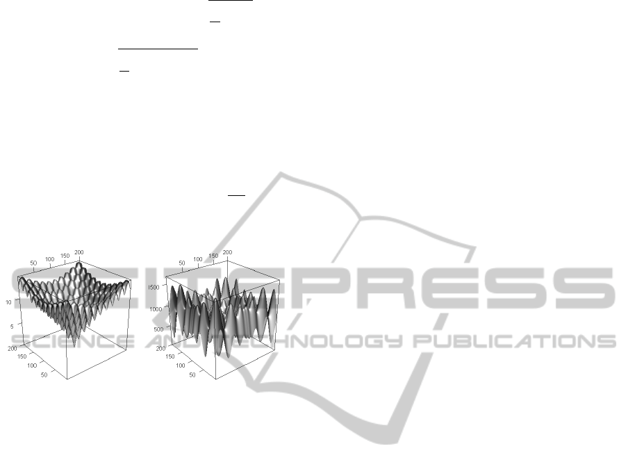
f (
−→
x ) = −20 exp
(
−0, 2 ·
s
1
D
D
∑
i=1
x
2
i
)
−exp
(
−0, 2 ·
s
1
D
D
∑
i=1
cos(2πx
i
)
)
+ 20 + e
(4)
Schwefel. The only used benchmark function whose
optimum is not at the coordinate origin. It is at
f (x
0..n
= 420.9687) = 0, and many local optima
exist (Rajasekhar et al., 2011).
f (
−→
x ) = 418.9829 · n −
n
∑
i=1
(x
i
sin(
p
|x
i
|)) (5)
Figure 5: Ackley and Schwefel benchmark functions.
4 EXPERIMENTAL SETUP
For the experiments covered in this paper a modified
version of the software tool introduced in (Bodenstein
and Zimmermann, 2014) was used. All mentioned
benchmark functions had to be implemented, includ-
ing calculation of actual optimum parameter set and
cost function value to evaluate the quality of the found
optima.
Two parameters were chosen, both discretized
with 10 000 steps. As a heuristic optimization run is a
stochastic experiment just like a single simulation run
itself, there is randomness in the computed run time
and accuracy. All optimization runs have thus been
tested 100 times and averaged to get trustworthy re-
sults. As base heuristic, Hill-Climbing was used for
all experiments. The idea is to apply a very simple al-
gorithm multiple times starting at a coarse discretiza-
tion and low simulation precision as the baseline.
As even simple Hill-Climbing implementations
can be widely configured, the used configuration
should be mentioned here. The algorithm calculates
the next value for every parameter by adding the min-
imum step size or discretization value. If this parame-
ter set results in a worse cost function value, an er-
ror counter is increased. Four worse solutions are
allowed before the next parameter is selected to be
changed. Optimization is stopped if five solutions in
a row are not better then a previously found parameter
set. Every parameter set resulting in a better solution
resets both error counters.
The number of worse solutions and worse solu-
tions per parameter are essential for tuning the heuris-
tic to overcome local optima.
Real SCPN simulations were not used in the
shown experiments. The mentioned benchmark func-
tions with different cost function shapes were used
instead. As these cost function shapes are similar
to known performance measure shapes of real SCPN
batch simulations or optimization models in general,
we assume that the results can be useful for simula-
tion based SCPN optimization.
5 RESULTS
The utilized heuristic (Hill-Climbing) was run 100
times, starting with random parameter sets for ev-
ery phase. The quality of a found optimum is de-
fined by the distance to a known absolute optimum
in value range and by the Euclidean distance in defi-
nition space.
Some results are shown in Table 1. The first and
most important result is the benefit of two phases for
slow steadily converging cost function shapes in terms
of result quality and needed simulation runs. The
benchmark functions Sphere and Matya represent this
kind of cost function. In this case, further increasing
the number of phases did not improve the result qual-
ity.
The optima quality of cost functions with sev-
eral local optima could be improved by increasing the
number of used optimization phases as shown in Ta-
ble 1, Figure 6, and Figure 7. Especially if many local
optima are expected, increasing the number of phases
does improve the quality of found optima.
The experimental results for Schwefel and Ackley
show dramatic improvements in terms of distance to
the known absolute optimum.
The resulting number of (pseudo-)simulations and
CPU time for optimization using multiple phases may
increase. However, even if the number of necessary
simulation runs for an optimization can not be re-
duced by applying more phases, the overall CPU time
for the complete optimization is effectively reduced.
It is depicted in figure 8. A number of 5 phases
seems to be the best choice for most types of func-
tion shapes.
SIMULTECH2015-5thInternationalConferenceonSimulationandModelingMethodologies,Technologiesand
Applications
98
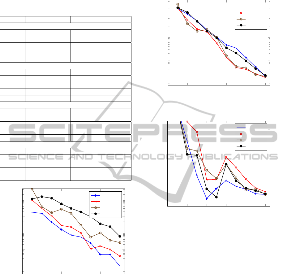
Table 1: Results of multi-phase optimization experiment
with benchmark function.
Phase-# Sim-# Dist. DS-Dist. CPU time
Sphere
1 2947.5 1.75% 19.74% 6976732.5
2 256.9 1.47% 10.83% 202660.7
3 171.5 0.44% 5.44% 55401.3
4 44.5 0.16% 2.16% 23450.5
10 72.2 0.00% 0.02% 27434.7
Matya
1 5056.1 9.29% 20.19% 1196778877
2 384.4 2.95% 5.97% 421244.4
3 622.0 1.05% 2.37% 283450.4
4 179.9 0.28% 1.82% 47842.9
10 87.6 0.00% 0.02% 30468.7
Ackley
1 570.2 42.61% 29.95% 1349663.4
2 102.0 3.73% 4.11% 153356.6
3 84.7 1.65% 1.89% 139848.7
4 53.2 2.64% 2.27% 68165.1
10 73.8 0.03% 0.02% 27459.3
Schwefel
1 295.8 10.95% 20.82% 700158.6
2 67.8 15.07% 13.06% 123082.9
3 82.2 12.14% 5.21% 118661.5
4 68.0 5.574% 1.917% 33708.5
10 76.8 0.06% 0.02% 28141.0
0 2 4
6
8 10
10
−3
10
−2
10
−1
10
0
10
1
Number of phases
Distance to optimum
Sphere
Matya
Ackley
Schwefel
Figure 6: Distance to optimum vs. Number of simulation
phases.
6 CONCLUSION
In this paper a multi-phase optimization approach in-
troduced in (Bodenstein and Zimmermann, 2015) was
extended to analyze the possible benefits in terms of
overall CPU time and result accuracy. To speed up the
experiments, the correlation between simulation pre-
cision and CPU time was examined and implemented
in benchmark functions as a substitute to real SCPN
simulations. Up to ten phases were tested in our ex-
0 2 4
6
8 10
10
−2
10
−1
10
0
10
1
Number of phases
Euklid distance to optimum (in DS)
Sphere
Matya
Ackley
Schwefel
Figure 7: Euclidian distance to optimum in definition space
vs. number of simulation phases.
0 2 4
6
8 10
10
4.5
10
5
10
5.5
Number of phases
CPU time
Sphere
Matya
Ackley
Schwefel
Figure 8: Phase count vs. CPU time.
periments.
Applying two phases increases the quality of the
found optima for all benchmark functions. When us-
ing more complex benchmark functions with several
local optima, increasing the number of phases leads to
better results and reduced CPU time in all considered
examples.
As many cost function shapes of SCPN perfor-
mance measures show several local optima, such a
multi-phase approach will improve CPU time and in-
crease the probability of finding the real optimum.
The paper presented first results to validate the gen-
eral hypothesis, but more experiments using real
SCPN simulations and other heuristics are currently
investigated. Another possibility for future research
is the extension of a heuristic such as Simulated An-
nealing with direct continuous simulation precision
control without using discrete phases.
ComputationallyEfficientMultiphaseHeuristicsforSimulation-basedOptimization
99

ACKNOWLEDGEMENTS
This paper is based on work funded by the Federal
Ministry for Education and Research of Germany un-
der grant number 01S13031A.
REFERENCES
Biel, J., Macias, E., and Perez de la Parte, M. (2011).
Simulation-based optimization for the design of dis-
crete event systems modeled by parametric Petri nets.
In Computer Modeling and Simulation (EMS), 2011
Fifth UKSim European Symposium on, pages 150–
155.
Bodenstein, C. and Zimmermann, A. (2014). TimeNET
optimization environment. In Proceedings of the 8th
International Conference on Performance Evaluation
Methodologies and Tools.
Bodenstein, C. and Zimmermann, A. (2015). Extend-
ing design space optimization heuristics for use with
stochastic colored petri nets. In 2015 IEEE Interna-
tional Systems Conference (IEEE SysCon 2015), Van-
couver, Canada. (accepted for publication).
Carson, Y. and Maria, A. (1997). Simulation optimization:
Methods and applications. In Proceedings of the 29th
Conference on Winter Simulation, WSC ’97, pages
118–126.
Fu, M. C. (1994a). Optimization via simulation: a review.
Annals of Operations Research, pages 199–248.
Fu, M. C. (1994b). A tutorial overview of optimization via
discrete-event simulation. In Cohen, G. and Quadrat,
J.-P., editors, 11th Int. Conf. on Analysis and Opti-
mization of Systems, volume 199 of Lecture Notes
in Control and Information Sciences, pages 409–418,
Sophia-Antipolis. Springer-Verlag.
Jamil, M. and Yang, X.-S. (2013). A Literature Survey of
Benchmark Functions For Global Optimization Prob-
lems. ArXiv e-prints.
K
¨
unzli, S. (2006). Efficient Design Space Exploration for
Embedded Systems. Phd thesis, ETH Zurich.
Rajasekhar, A., Abraham, A., and Pant, M. (2011). Levy
mutated artificial bee colony algorithm for global op-
timization. In Systems, Man, and Cybernetics (SMC),
2011 IEEE International Conference on, pages 655–
662.
Rodriguez, D., Zimmermann, A., and Silva, M. (2004). Two
heuristics for the improvement of a two-phase opti-
mization method for manufacturing systems. In Proc.
Int. Conf. Systems, Man, and Cybernetics (SMC’04),
pages 1686–1692, The Hague, Netherlands.
Sanders, W. H. and Meyer, J. F. (1991). A unified approach
for specifying measures of performance, dependabil-
ity, and performability. In Avizienis, A. and Laprie, J.,
editors, Dependable Computing for Critical Applica-
tions, volume 4 of Dependable Computing and Fault-
Tolerant Systems, pages 215–237. Springer Verlag.
Schoen, F. (2002). Two-phase methods for global optimiza-
tion. In Handbook of global optimization, pages 151–
177. Springer US.
Zenie, A. (1985). Colored stochastic Petri nets. In Proc. 1st
Int. Workshop on Petri Nets and Performance Models,
pages 262–271.
Zimmermann, A. (2007). Stochastic Discrete Event Sys-
tems - Modeling, Evaluation, Applications. Springer-
Verlag New York Incorporated.
Zimmermann, A. (2012). Modeling and evaluation of
stochastic Petri nets with TimeNET 4.1. In Perfor-
mance Evaluation Methodologies and Tools (VALUE-
TOOLS), 2012 6th Int. Conf. on, pages 54–63.
Zimmermann, A. and Bodenstein, C. (2011). Towards
accuracy-adaptive simulation for efficient design-
space optimization. In Systems, Man, and Cybernet-
ics (SMC), 2011 IEEE International Conference on,
pages 1230 –1237.
Zimmermann, A., Rodriguez, D., and Silva, M. (2001). A
two-phase optimisation method for Petri net models of
manufacturing systems. Journal of Intelligent Man-
ufacturing, 12(5/6):409–420. Special issue ”Global
Optimization Meta-Heuristics for Industrial Systems
Design and Management”.
SIMULTECH2015-5thInternationalConferenceonSimulationandModelingMethodologies,Technologiesand
Applications
100
