Norm Selection for Evaluation Criterion for Placement Planning of

Active Damping Devices in Structure

Kou Miyamoto

, Jinhua She

2,3

, Hiroshi Hashimoto

and Min Wu

Interdisciplinary Graduate School of Science and Engineering, Tokyo Institute of Technology,

4259 Nagatsuta-cho, Midori-ku, Yokohama, Kanagawa 226-8503, Japan

School of Engineering, Tokyo University of Technology, 1404-1 Katakura, Hachioji, Tokyo 192-0982, Japan

School of Automation, China University of Geosciences, Wuhan 430074, China

Master Program of Innovation for Design and Engineering, Advanced Institute of Industrial Technology

1-10-40 Higashiooi, Shinagawa-ku, Tokyo 140-0011, Japan

Keywords:

Active Damping Device (ADD), Active Vibration Control, Combinatorial Optimization, Norm, Placement

Planning.

Abstract:

Active vibration control has been widely investigated in civil engineering. This study considers the problem

of selecting a norm for an evaluation criterion for the planning of the placement of active damping devices

(ADDs) in a structure in active vibration control. Using a 4-degree-of-freedom system as an example, we

compare the commonly used 2-norm and ∞-norm, and show that the 2-norm is a suitable choice for the

performance index of the placement planning of ADDs.

1 INTRODUCTION

Since active structural control exhibits good control

performance, it has been attracting great attention. An

active structural control system has been designed us-

ing many control methods, for example, classical con-

trol (Gucu, 2006), modern control (She et al., 2010),

advanced control (Zhang et al., 2014), and predictive

control (Tsuji et al., 2012).

Due to the constraints on the cost and structure,

active damping devices (ADDs) have usually been

placed only on the top ﬂoor or at the base of the

structure. However, the situation has been changed in

the last decade. Along with the progress of the tech-

nologies in mechatronics in recent years, both of the

cost and the size of ADDs have been reduced greatly.

This provides ﬂexibility in the selection and place-

ment of an active structural control system (For ex-

ample, (Tokkyokiki Corporation, 2015)).

Take a four-story building as an example. An

ADD was placed on the ﬁrst ﬂoor in (Yoshida et al.,

1995), on the second ﬂoor in (Gucu, 2006), and on

all ﬂoors in (She et al., 2010). However, no explana-

tions for the placement were given. And it is ques-

tionable why they placed the ADDs in those way and

whether or not it is really necessary to place ADDs on

all ﬂoors. To solve these problems, we introduced the

2-norm of a control system to evaluate the control per-

formance (Miyamoto and She, 2015). In this study,

we extend the result in (Miyamoto and She, 2015) and

explore the commonly used norms for the purpose of

evaluating the placement planning of ADDs.

2 STRUCTURAL MODEL OF

4-STORY AND CONTROL

SYSTEM

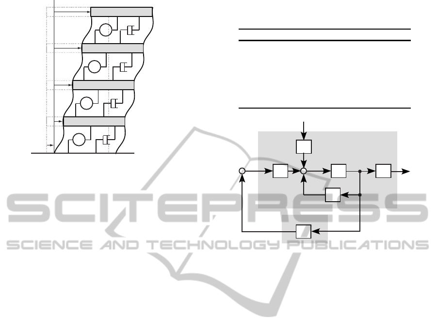
To make the discussion simple, we use a four-story

structure (Figure 1) in this paper. The achievedresults

can easily be extended to an n-story structure. The

motion of the system is described by

¨x(t) +C

˙x(t) + K

x(t) = E

u(t) + E

¨x

(t), (1)

where



x(t) = [x

(t), x

(t)]

u(t) = [ f

(t), f

(t)]

= diag{m

, m







+ c

−c

0 0

−c

+ c

−c

0 −c

+ c

−c

0 0 −c







117

Miyamoto K., She J., Hashimoto H. and Wu M..

Norm Selection for Evaluation Criterion for Placement Planning of Active Damping Devices in Structure.

DOI: 10.5220/0005520201170122

In Proceedings of the 12th International Conference on Informatics in Control, Automation and Robotics (ICINCO-2015), pages 117-122

ISBN: 978-989-758-122-9

 2015 SCITEPRESS (Science and Technology Publications, Lda.)

Figure 1: Dynamic model of four-story structure.







+ k

−k

0 0

−k

+ k

−k

0 −k

+ k

−k

0 0 −k













− b

0 0

0 b

− b

0 0 b

− b

0 0 0 b







= [m

, m

]

where the meanings of the parameters and variables

are given in Table 1. And E

indicates the placement

of ADDs, and b

(i = 1,2,3,4) in E

is given by



0, the ith ﬂoor does not have an ADD,

1, the ith ﬂoor has an ADD.

(2)

The state-space equation is



ξ(t) = Aξ(t) + Bu(t) + B

¨x

(t),

y(t) = Cξ(t),

(3)

where the state vector is ξ(t) =



(t), ˙x

(t)



, the

output is y(t) = x(t), and

A =



0 I

−M

−1

−M

−1



, B =



−M

−1





−E



, C =





, E = [1, 1, 1, 1]

In order to verify the relationship between the

placement of ADDs and control effect, it is necessary

to construct a control system. In this study, we con-

struct a simple optimal control system by minimizing

the following performance index

J =

∞



(t)Qξ(t) + u

(t)Ru(t)



dt, (4)

where Q (≥ 0) and R (> 0) are weighting matrices

such that (Q

1/2

,A) is observable. A feedback control

Table 1: Meanings of parameters and variables (i =

1,2,3, 4).

Symbol Meaning

[kg] Mass of the ith story

[Ns/m] Damping of the ith story

[N/m] Stiffness of the ith story

Displacement of the ith story

Output of the ith ADD

Displacement of the ground

d(t)

x(t)x(t)

Controller

s I

−1

Plant

u(t)

y(t)

Figure 2: Conﬁguration of optimal active-structural-control

system.

law is given by

u(t) = Kξ(t), (5)

K = −R

−1

P, (6)

P+ PA+ Q− PBR

−1

P = 0. (7)

As a result, the transfer function of the system from

the input to the output is

G(s) = C[sI − (A + BK)]

−1

B, (8)

where s is the operator of the Laplace transform. An

optimal state-feedback active-structural-control sys-

tem is shown in Figure 2.

3 SELECTION OF NORM FOR

PLANNING INDEX

First, we consider the norms for a signal. A norm of a

signal u(t) = [u

(t), u

(t), ·· · , u

(t)]

, kuk, has the

following properties:

1. kuk ≥ 0;

2. kuk = 0 ⇔ u(t) = 0, ∀t;

3. kauk = |a|kuk, ∀a ∈ R; and

4. ku + vk ≤ kuk + kvk .

ICINCO2015-12thInternationalConferenceonInformaticsinControl,AutomationandRobotics

118

Table 2: Relationships of the norms between input, output,

and system.

kuk

∞

pow(u)

kyk

kGk

∞

∞ ∞

kyk

∞

kGk

∞

pow(y) 0 ≤ kGk

∞

kGk

∞

1-norm, 2-norm, and ∞-norm of the signal are deﬁned

as follows.

kuk

∑

i=1

∞

−∞

(t)|dt, (9)

kuk



∞

−∞

(t)u(t)dt



1/2

, (10)

kuk

∞

= sup

(t)|. (11)

On the other hand, if

pow(u) =



lim

T→∞

−T

(t)u(t)dt



1/2

(12)

exist, we call the signal a power signal. Note that

a nonzero signal can have zero average power. So,

Property 2 does not hold for (12) and pow(·) is not a

norm.

For a stable system, G(s), its H

norm is

kGk



2π

∞

−∞

Trace

(− jω)G( jω)

dω



1/2



2πj

Trace{G

( ¯s)G(s)}ds



1/2

(13)

and its H

∞

norm is

kGk

∞

= sup

0≤ω≤∞

max

{G( jω)} . (14)

Note that, for a square matrix Φ = [φ

] ∈ C

n×n

Trace in (13) is Trace{Φ} =

∑

i=1

, and σ

max

(Φ) in

(14) is the maximum singular value of Φ.

The deﬁnitions of induced norms givethe relation-

ships of the norms between the input, u(t), the out-

put, y(t), and the system G(s) (Table 2) (Doyle et al.,

2009):

kGk

= sup

kuk

∞

6=0

kyk

∞

kuk

∞

, (15)

kGk

= sup

kuk

6=0

kyk

∞

kuk

, (16)

kGk

∞

= sup

kuk

6=0

kyk

kuk

= sup

pow(u)6=0

pow(y)

pow(u)

. (17)

It is clear from the above relationships that, to sup-

press the vibration caused by an earthquake and/or a

typhoon, it is suitable to use the 1-normor the ∞-norm

of the system from the disturbance to the output to

evaluate the effect caused by a disturbance, because

the worst output caused by the disturbances can be

evaluate by the 1- or ∞-norms of the system.

However, those norms may not be suitable for the

evaluation of the placement of active damping de-

vices. The reason is as follows. To suppress vibra-

tion quickly and efﬁciently, for a given control input

with limited power, the bigger the output produced by

the control input is, the more desirable the system is.

From this viewpoint, the use of the 2-norm of the sys-

tem from the control input to the output is suitable for

the planning of the placement of ADDs. We use a nu-

merical example to examine and this and compare the

use of norms in the next section.

Let k be the number of ADDs. The placement

problem is divided into two cases:

(1) k is not ﬁxed: The optimal problem is

max

∈{0,1}

kGk

. (18)

(2) k is ﬁxed: The optimal problem is

max

∈{0,1},

∑

i=1

kGk

. (19)

Note that these combinatorial optimization problems

are an integer programming problem, and can easily

be solved using well-known solvers.

4 NUMERICAL EXAMPLE

For simplicity, we only verify and compare the 2-

norm and ∞-norm of the system in this section.

The parameters of a four-story structure are

(Yoshida et al., 1995)







= 0.828, m

= m

= 0.842, m

= 0.640,

= 400, k

= 1600, k

= 1302, k

= 160,

= 7.5, c

= c

= 0.02.

(20)

For the design of a control system, the weighting ma-

trices in (4) were chosen to be

Q = 300× diag{100, 100, 100, 100, 1, 1, 1, 1}, R = I

(21)

where k is the number of ADDs.

This study used the ground acceleration data of

Noto Peninsula earthquake [Figure 3 (a) and (b)],

which has a low frequency, and Kobe earthquake

[Figure 3 (c) and (d)], which features randomness,

as disturbances in simulations (Japan Meteorological

Agency, 2015).

The peak-to-peak values (PPVs) of the maximum

displacements for Noto Peninsula earthquake for dif-

ferent placement plans of ADDs are shown in Table

NormSelectionforEvaluationCriterionforPlacementPlanningofActiveDampingDevicesinStructure

119

(a)

(c)

-400

-200

200

400

403020100

t [s]

[cm/s ] (Noto)

[cm/s ] (Kobe)

Spectrum (x 10

-3

)

400

300

200

100

Spectrum (x 10

-9

)

1086420

Frequency [Hz]

(b)

(d)

86420

Frequency [Hz]

-800

-400

400

50403020100

[s]

Figure 3: Input earthquake waves: (a) Noto Peninsula earthquake, (b) Power spectrum of Noto Peninsula earthquake; (c)

Kobe earthquake; and (d) Power spectrum of Kobe earthquake.

Table 3: Relationship between the placement of ADDs (up-

per row) and the PPV of the maximum displacement for

Noto Peninsula earthquake [cm] (lower row).

Sys1234 Sys123 Sys124 Sys12

7.27 (4F) 7.39 (4F) 7.66 (4F) 7.85 (4F)

Sys134 Sys13 Sys14 Sys1

7.98 (4F) 8.15 (4F) 8.50 (4F) 8.84 (4F)

Sys234 Sys23 Sys24 Sys2

11.36 (4F) 11.54 (4F) 11.95 (4F) 12.18 (4F)

Sys34 Sys3 Sys4

13.33 (4F) 13.65 (4F) 15.68 (4F)

3. In the table, the word in the parentheses in the

right column shows the place where the maximum

displacement occurred; and SysXYZ indicates that

the control system has ADDs at the X-th, Y-th, and

Z-th ﬂoors, for example, Sys1234 means that it has

ADDs at the ﬁrst to the fourth ﬂoors.

Tables 3 and 4 show that the ascending order of the

maximum PPV for the placement of ADDs is almost

the same for those two quite different earthquakes.

And Sys1 has the minimum PPV for the use of one

ADD, Sys12 is for two and Sys123 is for three ADDs.

Let PPV

(max)

SysN

be the maximum PPV of SysN. The

relative difference of the PPV for the placement of

ADDs is deﬁned to be

SysN

PPV

(max)

SysN

− PPV

(max)

Sys1234

PPV

(max)

Sys1234

× 100%. (22)

Table 4: Relationship between the placement of ADDs (up-

per row) and the PPV of the maximum displacement for

Kobe Peninsula earthquake [cm] (lower row).

Sys1234 Sys123 Sys124 Sys12

10.83 (4F) 11.02 (4F) 11.45 (4F) 11.81 (4F)

Sys134 Sys13 Sys234 Sys14

11.98 (4F) 12.25 (4F) 12.63 (4F) 12.86 (4F)

Sys1 Sys23 Sys24 Sys2

13.41 (4F) 20.34 (4F) 21.41 (4F) 21.90 (4F)

Sys34 Sys3 Sys4

23.79 (4F) 24.27 (4F) 29.17 (4F)

It is in the range of 2-56% for Noto earthquake and

2-17% for Kobe earthquake for three ADDs; in the

range of 8-83% for Noto earthquake and 9-120% for

Kobe earthquake for two ADDs; and in the range of

22-116% for Noto earthquake and 23-169% for Kobe

earthquake for one ADD. This clearly shows that,

while the increase of the ADDs improves the control

performance, suitable placement of ADDs also dra-

matically changes the control performance. Observ-

ing the above results yields the follows. First, since

the smallest difference of δ

SysN

between the use of

one and four ADDs for a suitable placement is about

22%, that between two and four is about 8%, and that

between three and four is about 2%; there is no need

to place ADDs at all ﬂoors. Second, the largest differ-

ence of δ

SysN

is as large as 146% for different place-

ment of the same number of ADDs. So, if we choose

ICINCO2015-12thInternationalConferenceonInformaticsinControl,AutomationandRobotics

120

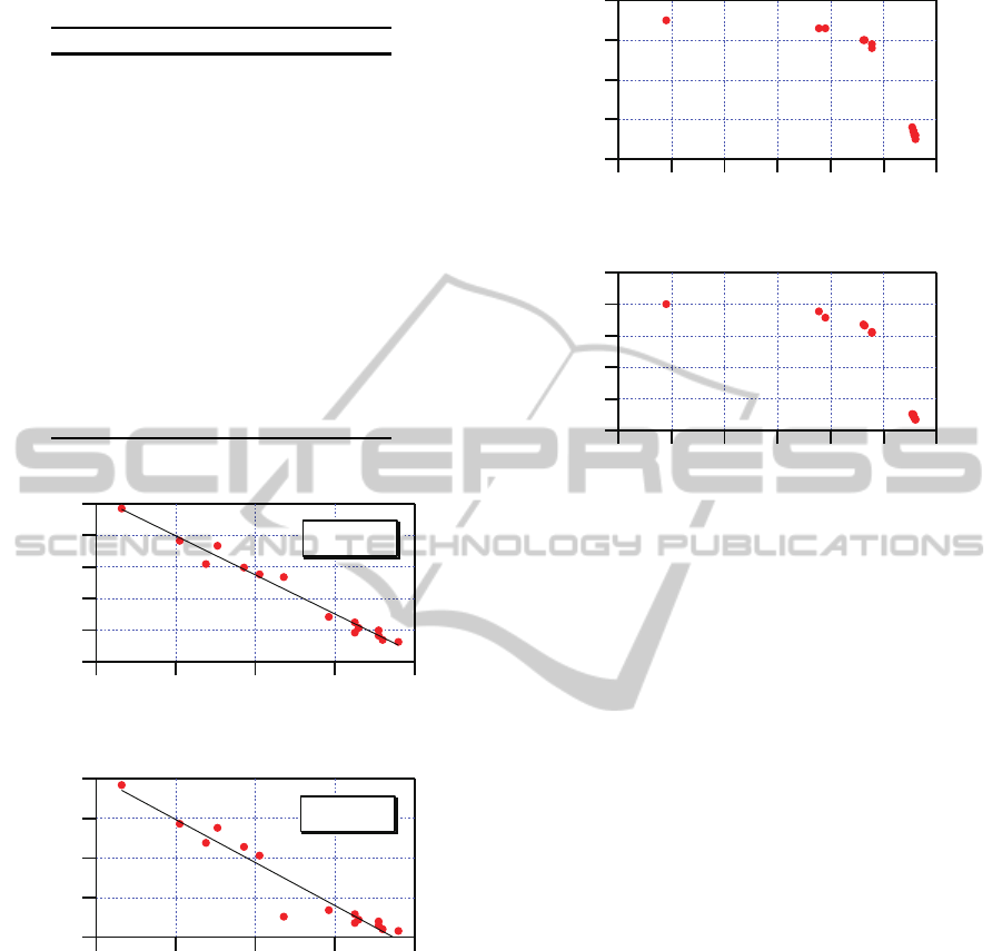
Table 5: Norms of active structural control system for (21).

Placement H

∞

Sys1234 0.01161 0.004301

Sys123 0.01118 0.004300

Sys134 0.01111 0.004282

Sys124 0.01109 0.004294

Sys13 0.01064 0.004281

Sys12 0.01054 0.004293

Sys14 0.01048 0.004275

Sys1 0.009854 0.004274

Sys234 0.008719 0.003894

Sys23 0.008106 0.003886

Sys24 0.007717 0.003819

Sys34 0.007048 0.003454

Sys2 0.006763 0.003805

Sys3 0.006102 0.003388

Sys4 0.004640 0.001951

(a)

(b)

Max. PPV dis. (Noto) [cm]

10864

G||

(x 1000)

= 0.9769

Max. PPV dis. (Kobe) [cm]

10864

G||

(x 1000)

= 0.9334

Figure 4: Relationship between the maximum PPV of the

output and the H

norm of the system for (a) Noto Peninsula

earthquake and (b) Kobe earthquake.

suitable ﬂoors to place devices, we can use a small

number of ADDs to achieve satisfactory aseismic ef-

fect.

Table 5 shows the calculated results of the H

and

∞

norms of G(s) for different placement of ADDs.

The relationships between the maximum PPV of the

output and the H

norm is shown in Figure 4, and

that between the maximum PPV and the H

∞

norm is

shown in Figure 5.

(a)

(b)

Max. PPV dis. (Noto) [cm]

4.5

4.03.53.02.52.01.5

G||

∞

(x 1000)

Max. PPV dis. (Kobe) [cm]

4.5

4.03.53.02.52.01.5

G||

∞

(x 1000)

Figure 5: Relationship between the maximum PPVs of the

outputs and the H

∞

norm of the system for (a) Noto Penin-

sula earthquake and (b) Kobe earthquake.

It is clear from Figures 4 and 5 that the maximum

PPV of the output is basically in inverse proportion to

the H

or H

∞

norms of the system. And all of the co-

efﬁcients of determination, R

, are larger than 0.9 in

Figure 4. However, the H

∞

norms of the system with

good control performance all almost have the same

value, 0.043, as shown in Table 5. Recall that the H

∞

norm of an SISO system is the peak gain value of its

Bode plot. It is easy to understand that the values be-

come almost identical when a vibration mode is sup-

pressed. As a result, if we use the H

∞

norm of the

system as a performance index to evaluate the place-

ment of ADDs, it may just show good control perfor-

mance for those disturbances with the frequency cor-

responding to the peak gain value of the Bode plot,

and does not guarantee the aseismic effect for distur-

bances with other frequencies. From this viewpoint,

we can say that it is not suitable to use the H

∞

norm of

a control system to evaluate the placement planning.

On the other hand, as shown in (13), the H

norm

of a control system is the square root of the area of its

frequency-response gain. It is basically different for

different placement of ADDs. So, it is suitable to use

the H

norm of the transfer function from the control

input to the output to evaluate the placement planning.

Another question is if the reduction of the number

of ADDs results in the increase of the power of the

control input of each ADD. To answer this question,

we plot the relationship between the maximum PPVs

NormSelectionforEvaluationCriterionforPlacementPlanningofActiveDampingDevicesinStructure

121

of the outputs and the 2-norms of the control inputs

for Kobe earthquake in Figure 6. The ﬁgure shows

that the power of the control input has no signiﬁcant

correlation. For example, Sys1 uses less input power

than Sys23 does, but it yields much better control per-

formance. So, good control performance produced by

the control system with a small number of devices,

which are given by the optimal placement (18), does

not mean the increase of control-input power. This

also shows the importance of the optimal placement

of ADDs.

Sys1

Sys14

Sys234

Sys13

Sys134

Sys12

Sys124

Sys123

Sys1234

Sys4

Max. PPV dis. (Kobe) [cm]

1.81.61.41.21.00.8

/ ||u

1234

}

Sys3

Sys34

Sys2

Sys24

Sys23

{

Figure 6: Relationship between the maximum PPVs of the

outputs and the 2-norms of the control inputs for Kobe

earthquake.

5 CONCLUSION

In this study, we considered the problem of the place-

ment of ADDs to perform active structural control.

To suitably evaluate the placement planning, we ex-

amined the 1-, 2-, and ∞-norms of a control system

from the control input to the output; and employed

the H

norm for the evaluation. We used a four-story

structure as an example to demonstrate the validity of

the selection. The following points were clariﬁed.

1. Increasing the number of ADDs does not neces-

sarily lead to the improvement of control perfor-

mance. Placing a small number of ADDs at suit-

able ﬂoors achieves satisfactory control result.

2. The H

norm of the transfer function from the

control input to the output is suitable for a per-

formance index to ﬁnd out an optimal placement

of ADDs.

ACKNOWLEDGEMENTS

This study was supported in part by the National

Natural Science Foundation of China under Grants

61473313 and 61210011; and by the Grant-in-Aid for

Scientiﬁc Research (C), Japan Society for the Promo-

tion of Science (JSPS) under Grant 26350673.

REFERENCES

Doyle, J., Francis, B., and Tannenbaum, A. (2009). Feed-

back Control Theory. Dover Publications, New York.

Gucu, R. (2006). Sliding mode and PID control of structural

system against earthquake. Mathematical and com-

puter modeling, 44:314-328.

Japan Meteorological Agency (2015) Mea-

sured data of severe earthquakes for

main earthquakes. [Online available]

http://www.data.jma.go.jp/svd/eqev/data/kyoshin/

jishin/index.html (accessed on 26 September, 2014)

Miyamoto, K. and She, J. (2015). Optimal Planning of Ac-

tuators in Structure Using H

Norm as Planning Index.

Transactions of the Japan Society of Mechanical En-

gineers Series C, (under review).

She, J., Sekiya, K., Wu, M., and Lei, Q. (2010). Ac-

tive Structural Control with Input Dead Zone Based

on Equivalent-Input-Disturbance Approach. In Proc.

of the 36th Annual conference of the IEEE Indus-

trial Electronics Society (IECON 2010), pages 47-52,

IEEE.

Tokkyokiki Corporation (2015). Vibration con-

trol Technology ω series. [Online available]

http://www.tokkyokiki.co.jp/product/product

o.html

(accessed on 26 September, 2014)

Tsuji, T., Nakamura, H., and Kagimura, S. (2012). Stud-

ies on an active preview control of structures and

applicability of predicted earthquake motions. Jour-

nal of Japan Society of Civil Engineers, Ser. A1

(Structural Engineering & Earthquake Engineering),

68:110-123.

Yoshida, K., Kang, S., and Kim, T. (1995). LQG Con-

trol and H

∞

Control of Vibration Isolation for Multi-

Degrees-of-Freedom Systems. Transactions of the

Japan Society of Mechanical Engineers Series C,

61:975-980.

Zhang, H., Wang, R., Wang, J., and Shi, Y. (2014). Ro-

bust ﬁnite frequency H

∞

static-output-feedback con-

trol with application to vibration active control of

structural systems. Mechatronics, 24:354-366.

ICINCO2015-12thInternationalConferenceonInformaticsinControl,AutomationandRobotics

122