
HVDC Line Parameters Estimation based on Line Transfer
Functions Frequency Analysis
Jocelyn Sabatier, Toni Youssef and Mathieu Pellet
IMS Laboratory, UMR 5218 CNRS, Bordeaux University, 351 cours de la Libération, 33405 Talence Cedex, France
Keywords: HVDC Line, Line Parameters Estimation.
Abstract: This paper proposes a method to estimate HVDC line parameters. After a reminder on the transfer functions
that characterise the dynamic behaviour of a DC line, link between these transfer functions resonance
frequencies and the line parameters is established. This link is then used to estimate the line parameters, the
resonance frequencies being determined using the power spectral density of voltage signals at the input and
output of the line. A numerical example highlights the efficiency of the proposed method.
1 INTRODUCTION
High-voltage direct current (HVDC) technology has
become a credible alternative for transmitting power
over long distances through submarine or
underground cable crossings (Hammons et al, 2000).
Indeed, the improvement of power electronics
devices has opened new perspectives for
transmission of electrical power through HVDC
links, which offer extra means to control power
flows in interconnected power systems or between
non synchronous areas.
HVDC links offers numerous environmental
benefits, including “invisible” power lines, neutral
electromagnetic fields and compact converter
stations. The power HVDC transmission line is one
of the major components of an HVDC electric
power system. Its major function is to transport
electric energy, with minimal losses, from the power
sources to the load centres, usually separated by long
distances. Losses are only 3% per 1000 km at a
standard cost (losses can be further reduced to 0.3%
for 1000 km, but at a higher cost). Possible
applications include:
- connecting wind farms to power grids,
- underground power links,
- providing shore power supplies to islands
and offshore oil & gas platforms,
- connecting asynchronous grids.
To ensure proper operation of an HVDC grid, a
control system must be implement with main
objectives (Bahrman and Johnson, 2007):
- control basic system quantities such as DC line
current, DC voltage, and transmitted power
accurately and with sufficient speed of response
- control higher-level quantities such as frequency in
isolated mode or provide power oscillation
damping to help stabilize the AC network
- ensure stable operation with reliable commutation
in the presence of system disturbances
- ensure proper operation with fast and stable
recoveries during AC system faults and
disturbances
- diagnose of the line integrity.
To reach these objectives, the controllers must
have an accurate knowledge of the HVDC line that
connect the grid node. This requires the
implementation of line parameters estimation
methods. Most of HVDC estimation methods found
in literature are purely numerical or signal based
methods that do not take into account the physical
particularities of long transmission lines (Zhou et al
2006) (Eriksson and Söder 2010), (Chetty and
Ijumba, 2011) (Cole, 2010) (Chakradhar and Ramu,
2007) (Xu and Fan, 2012) (Indulkar and
Ramalingam, 2008) (Yuan, 2009) (Wilson et al,
1999) (Grobler and Naidoo 2006). The goal of this
paper is to propose a different approch. After a
reminder on the transfer functions that characterise
the dynamic behaviour of a DC line, a relationship
between these transfer functions resonance
frequencies and the line parameters is established.
This relationship is then used to estimate the line
parameters, the resonance frequencies being
determined using the power spectral density of
497
Sabatier J., Youssef T. and Pellet M..
HVDC Line Parameters Estimation based on Line Transfer Functions Frequency Analysis.
DOI: 10.5220/0005521304970502
In Proceedings of the 12th International Conference on Informatics in Control, Automation and Robotics (ICINCO-2015), pages 497-502
ISBN: 978-989-758-122-9
Copyright
c
2015 SCITEPRESS (Science and Technology Publications, Lda.)

voltage signals at the input and output of the line. A
numerical example highlights the efficiency of the
proposed method.
2 HVDC LINE DYNAMICAL
MODEL AND RESONANCE
FREQUENCIES
2.1 Analytical Model of HVDC Lines
A HVDC transmission line can be characterized by
the following parameters (Chakradhar and Ramu
2007):
- line length: L
line
- line series resistance r and inductance l
- line shunt capacitance c and conductance g
The series resistance relies basically on the
physical composition of the conductor at a given
temperature. The series inductance and shunt
capacitance are produced by magnetic and electric
fields around the conductors, and depend on their
geometrical arrangement. The shunt conductance is
due to leakage currents flowing across insulators and
air. These parameters values determine the power-
carrying capacity of the transmission line and the
voltage drop across it at full load.
As shown by figure 1, the HVDC line dynamical
behavior can be modelled by a quadrupole F(s), that
links:
- V
e
: line input voltage,
- I
e
: line input current,
- V
s
: line output voltage,
- I
s
: line output current.
Figure 1: HVDC line model and connected load.
The HVDC line is connected to a load of
impedance Z(s) constituted of a resistance R
ch
in
parallel with a capacitor C
ch
, and thus:
sCR
R
sZ
chch
ch
1
.
(1)
Solution of the Telegraphist’s equation permits to
show that the currents and voltages at the HVDC
line terminals are linked by the relation
sI
sV
sF
sI
sV
e
e
s
s
(2)
With
line
c
line
linecline
Ls
sZ
Ls
LssZLs
sFsF
sFsF
sF
cosh
sinh
sinhcosh
2221
1211
(3)
and
csglsrsZ
lsrcsgs
c
.
(4)
If a load of impedance Z(s) is connected to the line,
then the following transfer functions can be
computed (among others):
linelinece
s
linelinee
s
LsLsssZsV
sI
LsLss
s
sV
sV
sinhcosh
11
sinhcosh
(5)
with
lsr
csg
sCR
R
sZ
sZ
s
chch
ch
c
1
.
(6)
The gain of transfer functions F
21
(s) and I
s
(s)/V
e
(s)
are plotted in figure 2, using the following realistic
numerical values for a HVDC line proposed in
(Teppoz, 2005):
L
line
= 300 (km), r = 3e
-2
(.km
-1
),
l = 1.05e
-3
(H.km
-1
), c = 11e
-9
(F.km
-1
)
g = 6.5e
-9
(
-1
.km
-1
), R
ch
= 200 (), C
ch
= 50e
-6
(F)
Figure 2, but also Figure 3, permit to highlight a
property: the zeros of F
21
(s) correspond to the
resonance frequencies
k
, k
N
*, of transfer
functions I
s
(s)/V
e
(s) and V
s
(s)/V
e
(s). The first
resonance
0
results in the load connected to the
line. The separation between
0
and
k
, kN* tie in
a well-built HVDC line since the bandwidth of the
line must be higher than the one of the load. This
property is now used to deduce a link between the
k
, kN.
2.2 Resonance Frequencies Link
The zero of transfer function F
21
(s) (or frequencies
k
, kN*), are the values of s = j
such that
0sinh
line
Ls
(7)
Z(s)
ICINCO2015-12thInternationalConferenceonInformaticsinControl,AutomationandRobotics
498
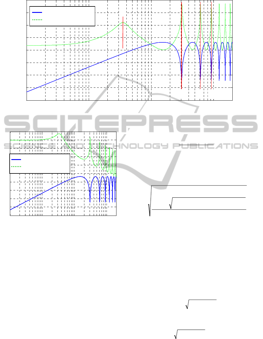
Figure 2: Comparison of F
21
(s) and I
s
(s)/V
e
(s) (with a load) gains.
Figure 3: Comparison of F
21
(s) and V
s
(s)/V
e
(s) gains.
or equivalently, the values of s = j
such that
ZkkLsm
Ls
line
line
I
Re
0
.
(8)
Using
jLs
line
(9)
and relation (4), then the following equality holds:
jLljrcjg
line
2
222
(10)
or
2
2
2222
line
line
Lglcr
Llcgr
(11)
thus leading to
2
2
line
Lglcr
(12)
and
044
2
2
22224
lineline
LglcrLlcgr
(13)
Solutions of equation (13) are:
2
2
22
2
2
22
glcrLlcgrL
Llcgr
lineline
line
(14)
The first equation of relation (8) is met if
2
22
2
2
2
2
2
glcrLlcgr
Llcgr
line
line
. (15)
It can be deduced that
= 0 is a solution of relation
(15). For the second equation of (8) with the
condition
=0, relation (10) can be rewritten as:
222
line
Llcgr
, (16)
and thus
2
lcgrL
line
. (17)
The frequencies
k
that met the second equation of
(8) are defined by
klcgrL
line
2
, (18)
and thus
10
1
10
2
10
3
10
4
-90
-80
-70
-60
-50
-40
-30
-20
-10
Frequency (rd/s)
Gain (dB)
F
21
(s) without load
F
21
(s) with load
0
2
3
1
10
1
10
2
10
3
10
4
-90
-80
-70
-60
-50
-40
-30
-20
-10
0
10
Frequency (rd/s)
Gain (dB)
F
21
(s)
I
s
(s)/V
e
(s) with a load
F
21
(s)
V
s
(s)/V
e
(s) with a load
HVDCLineParametersEstimationbasedonLineTransferFunctionsFrequencyAnalysis
499

grk
L
lc
line
k
2
2
2
1
with
Nk
. (19)
2.3 First Resonance Frequencies
To evaluate the first resonance frequency
0
, a one
cell -model of the line is considered. This model is
represented by figure 4 with
lineline
lineline
lLLcLC
gLGrLR
. (20)
Figure 4: One cell -model connected to a load Z(s).
Using Kirchhoff’s laws, it can be demonstrated that:
ssZ
C
sZ
G
LsRsZ
sI
sV
s
e
22
1
(21)
After simplifications, the transfer function
I
s
(s)/V
e
(s) is given by
2
00
1
0
21
1
s
s
s
C
sU
sI
e
s
(22)
with
CCLR
RGRRR
chch
chch
2
22
0
. (23)
The first frequency resonance in figure 2 or figure 3
can thus be approximated by relation (23).
2.4 Steady State Analysis
To study the line steady state behavior, the -model
of figure 4 is considered again.
In steady state, the inductance L acts as a thread
and the capacitor behaves like an open circuit. The
linear resistance is of the order of 10
-2
.km
-1
and
the linear conductance is of the order of 10
-9
S.km
-1
.
The product RG is thus very small and the following
simplification can be done:
e
se
I
VV
R
e
se
U
II
G
(24)
The lineic resistance and conductance of the line can
be deduced using relations (20) using steady state
(of low pass filtered) measures of line input and
output currents and voltages.
3 LINE PARAMETERS
ESTIMATION
The goal of this part is to show how to deduce line
parameters r, l, c, g from the knowledge of
frequencies
k
, kN, resulting in the measures of
voltages and currents at the line terminals.
With frequencies
k
and
k+1
given by relation
(19), the following equations can be obtained:
2
2
2
2
1
1 k
L
grlc
line
k
(25)
and
2
2
2
2
k
L
grlc
line
k
. (26)
Thus, using
2
line
k
L
kK
(27)
the following products are obtained using relation
(26) with k=1 and k=2:
2
1
2
2
1
2
22
2
1
KK
gr
and
2
1
2
2
12
KK
lc
. (28)
The line’s length being considered known, if the
second and the third resonance frequencies (ω
1
and
ω
2
) are known, the products lc and gr can be
deduced from equation (28).
Let’s consider the relation (23) which can be
rewritten as
linechlinech
chlinelinech
cLClLR
RrgLrLR
2
22
2
2
0
(29)
and thus using relation (28) for the product lc:
chlinelinech
linechlinechch
RrgLrLR
KK
LRlLCR
2
2
1
2
2
12
22
0
2
0
22
2
. (30)
Z(s)
R
L
C/2 G/2
C/2
G/2
I
e
(s)
I
s
(s)
V
e
(s)
V
s
(s)
-model
ICINCO2015-12thInternationalConferenceonInformaticsinControl,AutomationandRobotics
500

The value of l is thus given by
linechch
linechchlinelinech
LCR
KK
LRRrgLrLR
l
2
0
2
1
2
2
12
22
0
2
2
22
(31)
Now, from relation (28), the value of c is given by
2
1
2
2
12
1
KK
l
c (32)
To summarize, the line length L
line
being
considered known, parameter r can be deduced
from equations (24) and (20). Then from the first
three resonance frequencies (ω
0
, ω
1
and ω
2
),
parameters g, c and l can be deduced from
equations (28), (31) and (32).
4 APPLICATION USING POWER
SPECTRAL DENSITY
Power Spectral Density (PSD) is now used to
evaluate the first three resonance frequencies of the
transfer function V
s
(s)/V
e
(s). A 100 km length
HVDC line is considered. This line is characterized
by the parameters given in (Teppoz, 2005) and
gathered in table 1.
A voltage pulse input is applied to the line
(similar to a line disturbance). The resulting voltage
output is represented by figure 5. Noise has been
voluntarily added to the signals.
The PSD of the output voltage is then estimated
and represented on figure 6. Figure 6 exhibits three
spikes which correspond to the first three resonance
frequencies of the Bode diagram of V
s
(s)/V
e
(s)
transfer function. The aim is now to obtain the value
of the three frequencies. For that, the variance of the
spectrum is calculated using a sliding window of 8
samples. A variance signal of the same length of the
spectrum signal is obtained and plotted on figure 7.
Table 1: Considered HVDC line parameters.
Parameter Value
L
line
100 (km)
r
3
(.km
-1
)
l
1.05
(H.km
-1
)
11
(F.km
-1
)
6.5
(
-1
.km
-1
)
200
()
50
(F)
Figure 5: Time response of the system to a pulse input.
Figure 6: Power Spectral Density of the output of the
system in response to a step input.
A threshold test is finally applied on the variance
signal to obtain an estimation of the resonance
frequencies. They are compared with the exact
frequencies in table 2. In steady state, for V
e
(t)
=10
5
V, then V
s
(t) 9.57e
4
V, I
e
(t) 479.7A and
I
s
(t) 478.6A. Using relations (23) and (19), the
estimated line resistance r is thus 2.9e
-2
.km
-1
leading to a relative error of 3% and g is estimated
equal to 3.6779e-008
-1
.km
-1
thus estimated with
an error of 464%. Finally, relations (31) and (32)
provide c = 1.156e
-6
F and l = 0.10207 H. The
estimation errors are respectively 4.3 % and 2.8%.
The large estimation error for parameter g is a result
of its very small value (very accurate voltages and
currents measures with many decimals are required
to estimate a so small value). But this error has no
impact on the line dynamic behaviour.
0 0.02 0.04 0.06 0.08 0.1 0.12 0.14 0.16 0.18 0.2
9.4
9.6
9.8
10
10.2
x 10
4
Time (s )
V
s
Voltage (V)
0 0.02 0.04 0.06 0.08 0.1 0.12 0.14 0.16 0.18 0.2
1
1.2
1.4
1.6
1.8
x 10
5
Time (s )
V
e
Voltage (V)
0 0.5 1 1.5 2 2.5 3
0
5
10
15
20
25
30
35
40
45
Frequency (kHz)
Power/frequency (dB/Hz)
py
HVDCLineParametersEstimationbasedonLineTransferFunctionsFrequencyAnalysis
501

Figure 7: Variance signal of the spectrum of the output.
Table 2: Estimated resonance frequencies.
Frequencies Exact (Hz) Estimated (Hz)
0
68.5 70.3
1
1475 1477
2
2945 2930
5 CONCLUSIONS
This paper proposes an approach for HVDC line
parameters estimation. This method exploits the
voltage information at the input and the output of the
line. Using power spectral density computation the
first three resonance frequencies of the transfer
function linking the line input and the output voltage
are obtained. Through a theoretical analysis of the
line transfer functions, a link has been demonstrated
between the resonance frequencies and the line
parameters. The line steady state behaviour is finally
used to obtain the numerical values of the line
parameters the others being obtained using
resonance frequencies estimation. This method
differs from other methods presented in the literature
by its frequency and physical approach. In future
work, the authors intend now to propose another
method permitting the computation of resonance
frequencies using a fractional transfer function.
ACKNOWLEDGEMENTS
This research is supported by the French national
project WINPOWER ANR-10-SEGI-016.
REFERENCES
Hammons T. J., Woodford D., Loughtan J., Chamia M., J.
Donahoe J., Povh D., Bisewski B. and Long W., 2000.
Role of HVDC Transmissions in Future Energy
Development, IEEE Power Engineering Review, pp.
10-25.
Bahrman M. P. and Johnson B. K., 2007. The ABCs of
HVDC Transmission Technologies”. IEEE power &
energy magazine, pp. 32-44.
Zhou N., Pierre J. W. and Hauer J. F. 2006 , Initial Results
in Power System Identification From Injected Probing
Signals Using a Subspace Method", IEEE
Transactions on power systems, Vol. 21, No. 3.
Eriksson R. and Söder L., 2010. Coordinated control
design of multiple HVDC links based on model
identification, Computers and Mathematics with
Applications 60, pp 944-953.
Chetty L. and Ijumba N.M. 2011, System Identification Of
Classic HVDC Systems, South African Institute Of
Electrical Engineers, Vol.102 (4).
Cole S., 2010. Steady-State and Dynamic Modeling of
VSC HVDC Systems for Power System Simulation,
PhD thesis, Université catholique de Louvain,
Belgium.
Chakradhar R. Ch. and Ramu T. S. 2007, Estimation of
Thermal Breakdown Voltage of HVDC Cables - A
Theoretical Framework, IEEE Transactions on
Dielectrics and Electrical Insulation Vol. 14, No. 2.
Xu L. and Fan L., 2012, System Identification based VSC-
HVDC DC Voltage Controller Design, IEEE North
American Power Symposium.
Indulkar C. S., Ramalingam K., (2008) Estimation of
transmission line parameters from measurements,
International Journal of Electrical Power & Energy
Systems, Volume 30, Issue 5, Pages337-342.
Yuan L., 2009. Some Algorithms for Transmission Line
Parameter Estimation, 41st Southeastern Symposium
on System Theory,Tullahoma, TN, USA.
Wilson R. E., Zevenbergen G. A., Mah D. L., Murphy A.
J., (1999). Calculation of transmission line parameters
from synchronized measurements” Electric Machines
and Power Systems, 27:1269-1278.
Grobler M. and Naidoo R. (2006). Determining
transmission line parameters from gps time-stamped
data, Paris, Proceeding of the 32nd Industrial
Electronics conference.
Teppoz L (2005). Commande d’un système de conversion
de type VSC-HVDC Stabilité - Contrôle des
perturbations. PhD thesis, Institut National
Polytechnique de Grenoble.
0 50 100 150 200 250 300
0
200
400
600
800
1000
1200
1400
Variance
Sample number
ICINCO2015-12thInternationalConferenceonInformaticsinControl,AutomationandRobotics
502
